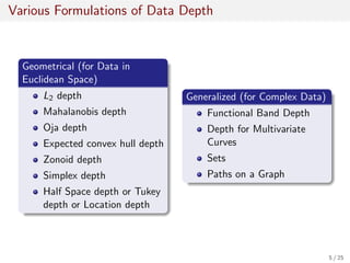
This document discusses generalized notions of data depth that can be applied to complex data types beyond traditional multivariate data. It describes formulations of data depth for functions, multivariate curves, sets, and paths on graphs. Data depth measures how deep or central a data point is within a data distribution. Generalized formulations allow data depth analysis of complex data like time series, curves, contours, and network paths. Visualization techniques like boxplots and bands are also discussed to illustrate the data depth of elements within ensembles of complex data.

1. Generalized Notions of Data Depth
Spring 2015 Data Reading Seminar
Mukund Raj
12th Mar, 2015
1 / 25

2. Outline
1 Data Depth Background
What is Data Depth?
Geometrical Data Depth
General Properties of Data Depth
2 Generalized Notions of Data Depth
Functions
Multivariate Curves
Sets
Paths (on a graph)
3 Discussion
Relaxed Formulations
Advantages and Limitations of Data Depth
2 / 25

3. What is Data Depth?
A means of measuring how deep a data point p is within a
cloud of points {p1, . . . , pn}.
Multivariate data analysis approach to generate order statistics
which capture high-dimensional features and relationships.
Descriptive nonparametric method of statistical analysis.
3 / 25

4. Why is Data Depth Interesting?
Estimate the location from center outward ( with respect to
parent distribution ).
Identify outliers.
Formulate quantitative and graphical methods for analyzing
distributional characteristics such as location, scale, e.t.c as
well as hypothesis testing.
Robustness.
4 / 25

5. Various Formulations of Data Depth
Geometrical (for Data in
Euclidean Space)
L2 depth
Mahalanobis depth
Oja depth
Expected convex hull depth
Zonoid depth
Simplex depth
Half Space depth or Tukey
depth or Location depth
Generalized (for Complex Data)
Functional Band Depth
Depth for Multivariate
Curves
Sets
Paths on a Graph
5 / 25

6. Geometrical data depth
Depth based on distances / volumes
L2 depth
Mahalanobis depth
Oja depth
Depth based on weighted means
Zonoid depth
Expected Convex Hull depth
Depth based on half spaces and simplices
Tukey depth
Simplicial depth
[Mosler 2012]
6 / 25

7. General Properties of Data Depth
1 Zero at infinity
2 Maximality at Center
3 Monotonicity
4 Affine Invariance
[Zuo and Serfling, 2000]
7 / 25

8. Outline
1 Data Depth Background
What is Data Depth?
Geometrical Data Depth
General Properties of Data Depth
2 Generalized Notions of Data Depth
Functions
Multivariate Curves
Sets
Paths (on a graph)
3 Discussion
Relaxed Formulations
Advantages and Limitations of Data Depth
8 / 25

9. Function Ensembles
A function ensemble can be defined as:
{xi (t), i = 1, . . . , n, t ∈ I} where I is an interval in and
xi : →
Time series observations annual trend of temperature or
precipitation, prices of commodities, heights of children versus
age e.t.c.
9 / 25

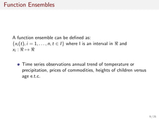
10. Motivation for Functional Band Depth
Challenge with regular multivariate analysis of functions
Curve ensembles that are sampled at different points.
Curse of dimensionality in case of current methods (e.g.
PCA).
Contribution by [L´opez-Pintado et. al. 2009]
Given an ensemble of functions (sampled from a distribution),
a formulation of data depth associated with the function.
10 / 25

11. Functional Band Depth Formulation
Figure: A functional band [Lopez-Pintado et. al. 2009].
Functional band formulation:
g ⊂ B(f1, · · · , fj ) iff ∀x min
i∈{1...j}
{fi(x)} ≤ g(x) ≤ max
i∈{1...j}
{fi(x)}
(1)
Functional band depth formulation:
BDj (g) = P (g ⊂ B(f1, · · · , fj)) (2)
11 / 25

12. Visualization of Data Depth for Functions
Figure: Visualization of function
ensemble [Lopez-Pintados et. al.
2009].
Figure: Boxplot visualization of
function ensemble [Sun et. al. 2011,
Whitaker et. al. 2013].
12 / 25

13. Multivariate Curve Ensembles
A parameterized curve can be defined in terms
of an independent parameter s as:
c(s) = ˜x(s) c : D → R D ⊂ R, R ⊂ Rd
Hurricane paths.
Brain tractography data.
Pathline ensemble in fluid simulation. Figure: A synthetic
ensemble of
multivariate curves in
[Mirzargar et. al.
2014]
13 / 25

14. Data Depth Formulation for Multivariate Curves
(a) (b)
Figure: Band formed by 3 multivariate curves [Lopez-Pintado et. al.
2014, Mirzargar et. al. 2014]
Curve band formulation:
g ⊂ B(ci1 , · · · , cij
) iff ∀x g(x) ∈ simplex ci1 (x), · · · , cij (x)
(3)
Curve band depth formulation:
SBDj (g) = P g ⊂ B(fc1 , · · · , cij ) (4)
14 / 25

15. Visualization of Data Depth for Curves
Figure: Chinese Script replicated
100 times [Lopez-Pintado 2014].
Figure: Curve boxplot for hurricane
path ensemble [Mirzargar et. al.
2014]
15 / 25

16. Set / Isocontour Ensembles
Given an ensemble of real valued functions
f (x, y), the sublevel and superlevel sets for any
particular isovalue.
Isocontours of temperature field.
Isocontours of pressure field in fluid
dynamics simulations.
Figure: A synthetic
ensemble of contours
in [Whitaker et. al.
2013]
16 / 25

17. Data Depth Formulation for Sets
Figure: Examples of set band [Whitaker et. al. 2013]
Set band formulation:
S ∈ sB(S1, . . . , Dj ) ↔
j
k=1
Sk ⊂ S ⊂
j
k=1
Sk (5)
Set band depth formulation:
sBDj (S) = P (S ⊂ sB(S1, . . . , Sj ) (6)
17 / 25

18. Visualization of Data Depth for Sets
(a)
(b)
Figure: Contour boxplot for an ensemble of isocontours of pressure field
[Whitaker et. al. 2013]
18 / 25

19. Paths (on a graph)
Let G = {V , E, W }. A path p can be denoted
as p : I → V where index set I = (1, . . . , m)
Paths of packets in computer networks.
Paths on transportation networks
modelled as graphs.
Figure: A synthetic
ensemble of paths on
a graph.
19 / 25

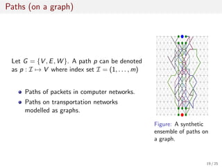
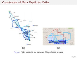
20. Data Depth Formulation for Paths
Figure: Illustration of band formed by 3 paths.
Path band formulation:
p ∈ B[Pj ] iff p(l) ∈ H[p1(l), . . . , pj (l)] ∀l ∈ I (7)
Path band depth formulation:
pBDj (p) = E [χ(p ∈ B(pj ))] (8)
20 / 25

21. Visualization of Data Depth for Paths
(a) (b)
Figure: Path boxplots for paths on AS and road graphs.
21 / 25

22. Outline
1 Data Depth Background
What is Data Depth?
Geometrical Data Depth
General Properties of Data Depth
2 Generalized Notions of Data Depth
Functions
Multivariate Curves
Sets
Paths (on a graph)
3 Discussion
Relaxed Formulations
Advantages and Limitations of Data Depth
22 / 25

23. Relaxed formulations
1 Modified Band Depth - Instead of an indicator function,
measure object inside the band.
2 Subsets - Indicator function with a relaxed threshold.
23 / 25

24. Advantages and Limitations
For Combinatorial Data Depth Formulations for Complex Data
Advantages
No assumption required for the underlying distribution.
Captures nonlocal relationships
Robust.
Limitations
Computationally expensive for large ensembles.
24 / 25

25. Thank You
Questions?
25 / 25