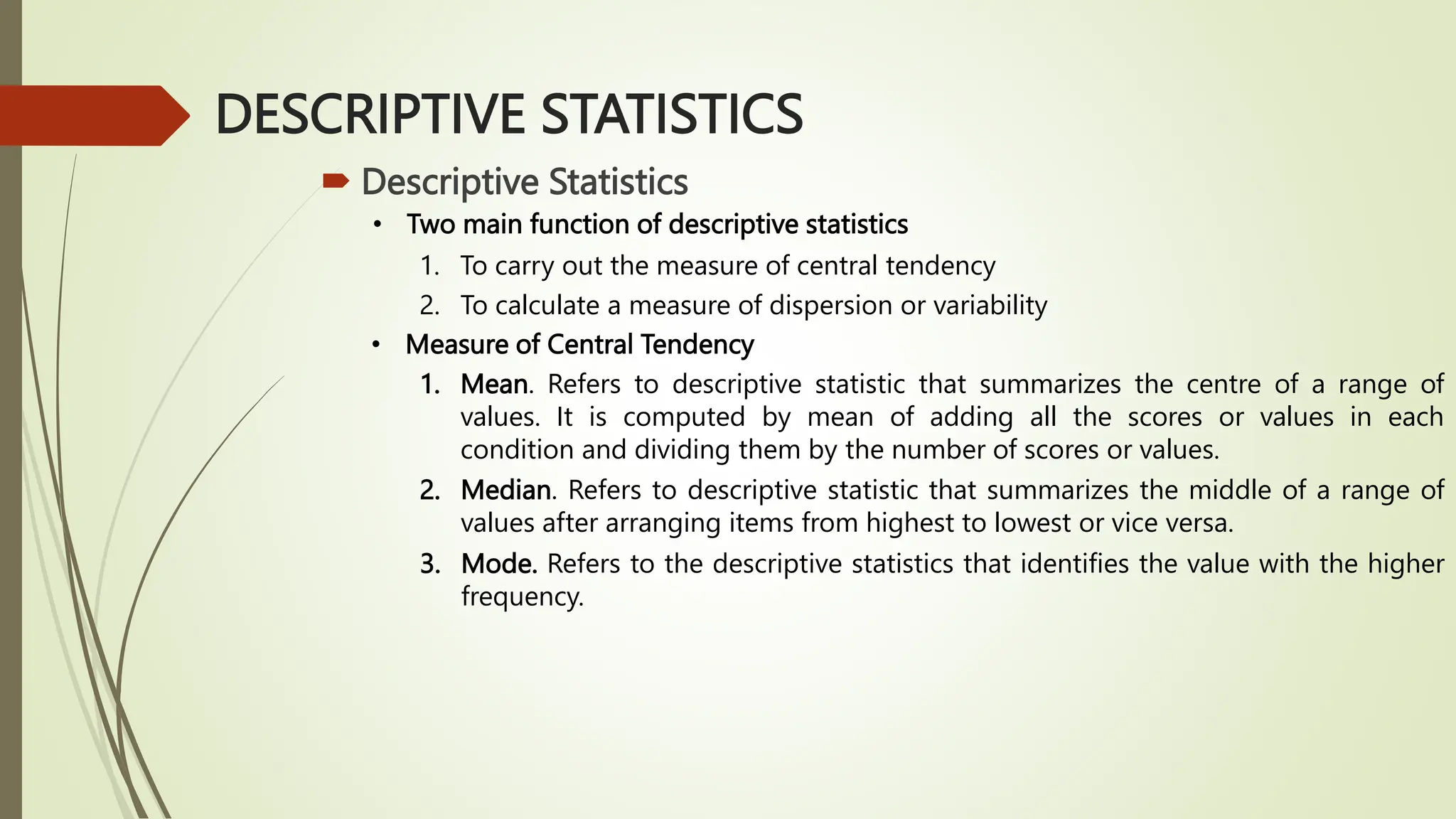
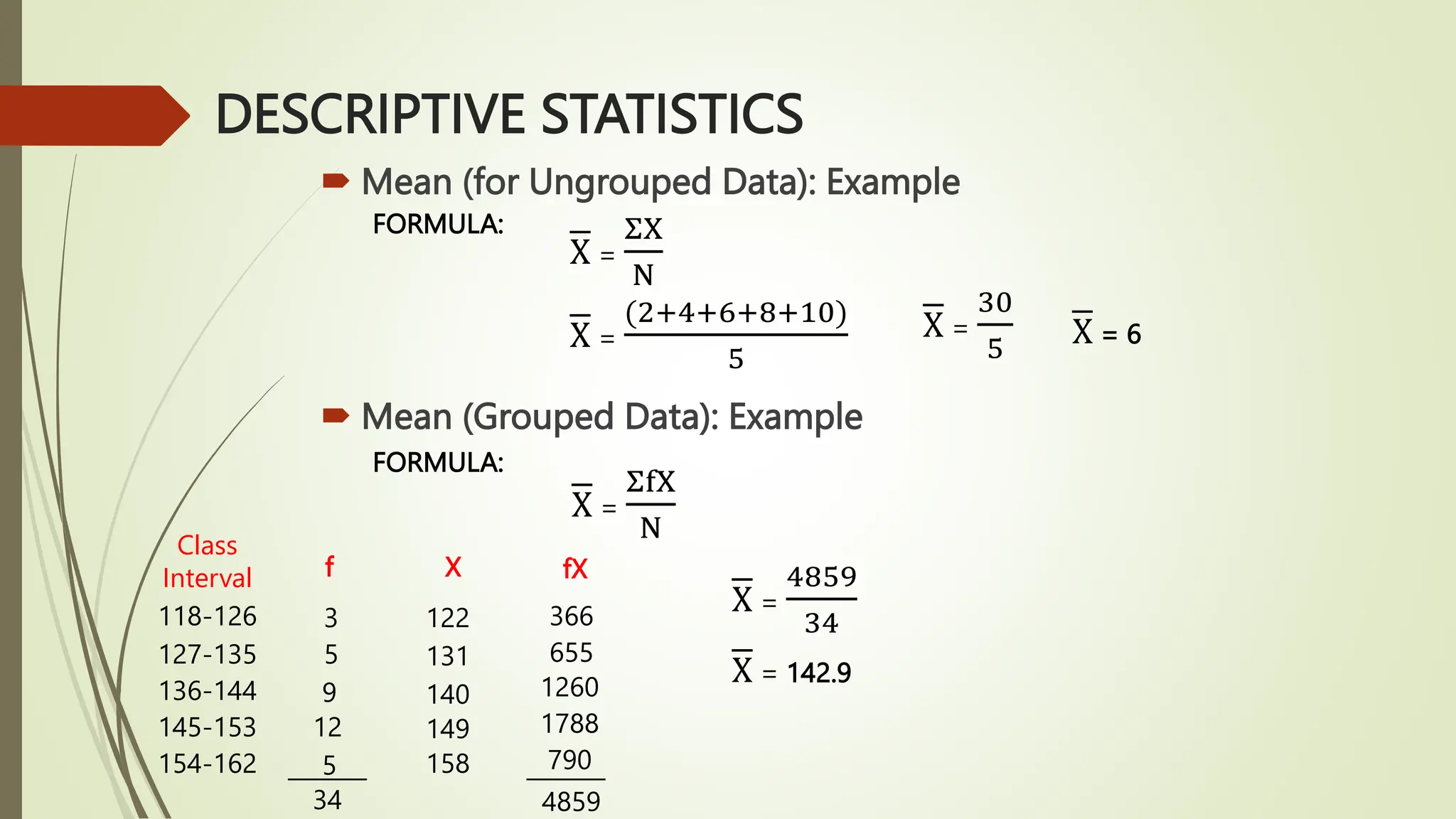
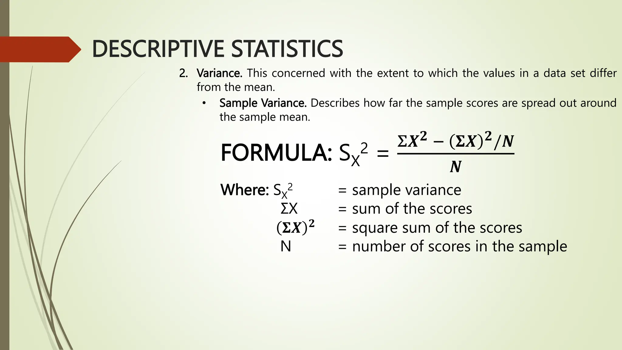
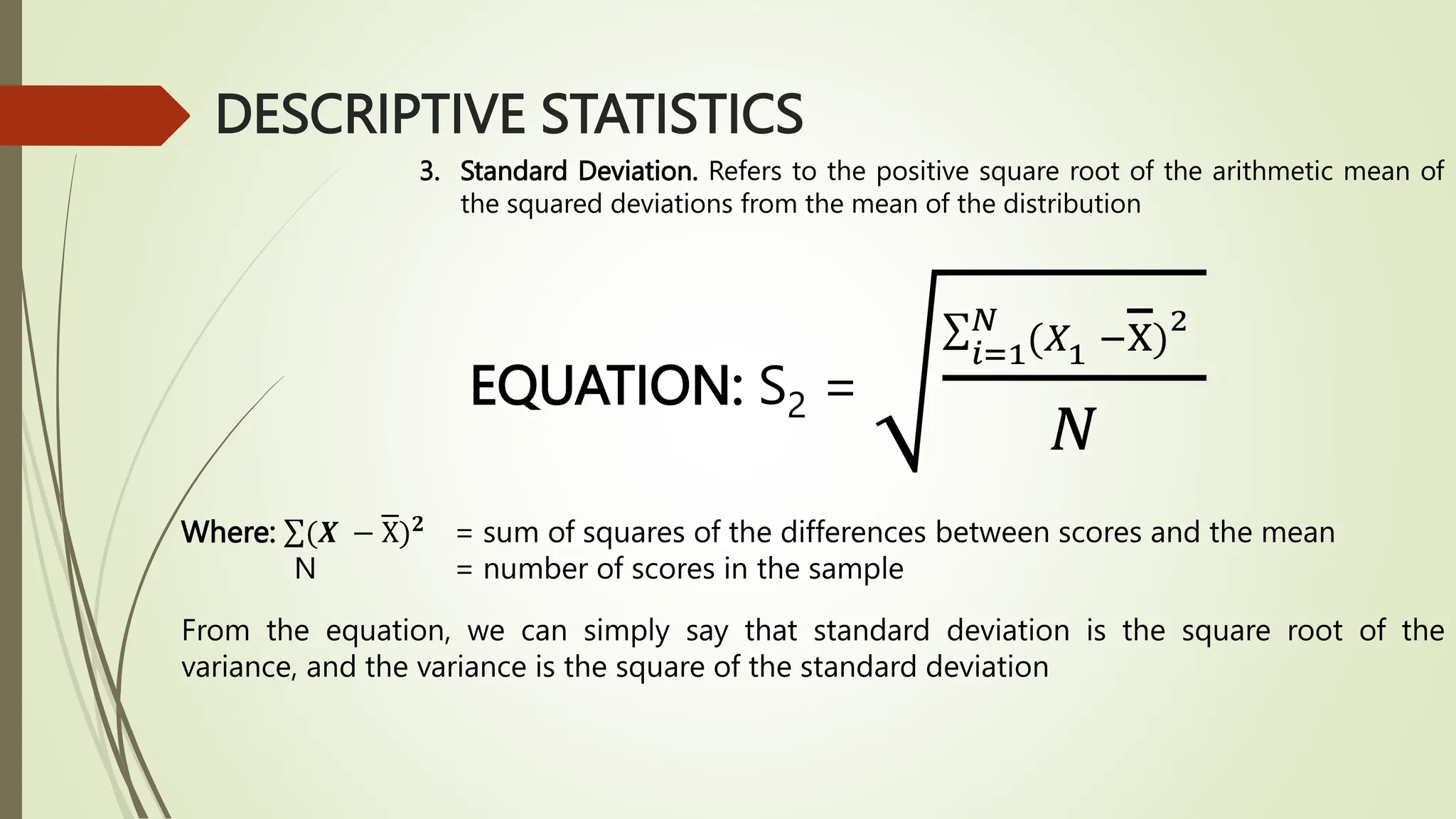
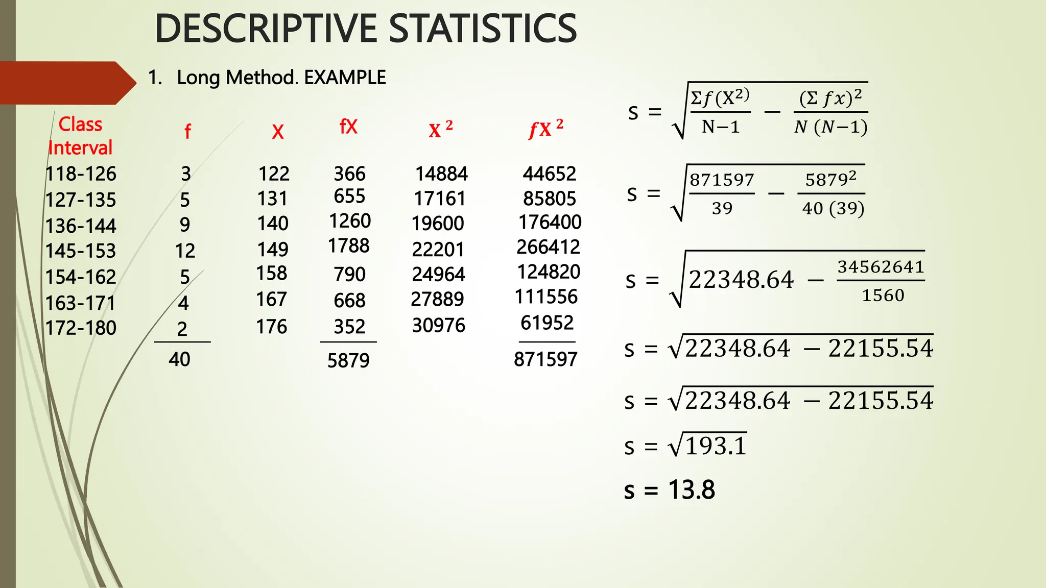
2. DESCRIPTIVE STATISTICS
ο΄ Descriptive Statistics
β’ Two main function of descriptive statistics
1. To carry out the measure of central tendency
2. To calculate a measure of dispersion or variability
β’ Measure of Central Tendency
1. Mean. Refers to descriptive statistic that summarizes the centre of a range of
values. It is computed by mean of adding all the scores or values in each
condition and dividing them by the number of scores or values.
2. Median. Refers to descriptive statistic that summarizes the middle of a range of
values after arranging items from highest to lowest or vice versa.
3. Mode. Refers to the descriptive statistics that identifies the value with the higher
frequency.
3. 10 13 13 22 23 25 30 35 40
β’ Example
Mean =
10+ 13+13+22+23+25+30+35+40
9
=
211
9
= 23.44
Median = 23
β’ RULES:
ο If N is an ODD NUMBERS, get the EXACT MIDDLE SCORE/NUMBER
ο If N is an EVEN NUMBERS, get the AVERAGE OF TWO MIDDLE
SCORES/NUMBERS
Mode = 13
DESCRIPTIVE STATISTICS
4. β’ Illustration of the Rules in the Median
ο If N is an ODD NUMBERS, get the EXACT MIDDLE SCORE/NUMBER
ODD NUMBERS: 5 10 15
Median = 10
ο If N is an EVEN NUMBERS, get the AVERAGE OF TWO MIDDLE
SCORES/NUMBERS
EVEN NUMBERS: 2 4 6 8
Median =
4 + 6
2
Median = 5
DESCRIPTIVE STATISTICS
5. ο΄ Mean (for Ungrouped Data): Example
FORMULA:
X =
Ξ£X
N
X =
(2+4+6+8+10)
5
X =
30
5 X = 6
ο΄ Mean (Grouped Data): Example
FORMULA:
X =
Ξ£fX
N
Class
Interval
118-126
127-135
136-144
145-153
154-162
f
3
5
9
12
5
_______
34
X
122
131
140
149
158
fX
366
655
1260
1788
790
_______
4859
X =
4859
34
X = 142.9
DESCRIPTIVE STATISTICS
6. β’ Measure of Dispersion
1. Range. Refers simply the highest value minus the lowest value
FORMULA: Range ( R ) = Highest Score (HS) β Lowest Score (LS)
ο EXAMPLE:
50 60 10 25 25 30 20 40
R = HS β LS
= 60 β 10
= 50
2 3 4 5 6 7 8 9
R = HS β LS
= 9 β 2
= 7
DESCRIPTIVE STATISTICS
7. 2. Variance. This concerned with the extent to which the values in a data set differ
from the mean.
β’ Sample Variance. Describes how far the sample scores are spread out around
the sample mean.
FORMULA: SX
2 =
Ξ£πΏπ β πΊπΏ π/π΅
π΅
Where: SX
2 = sample variance
Ξ£X = sum of the scores
πΊπΏ π = square sum of the scores
N = number of scores in the sample
DESCRIPTIVE STATISTICS
9. β’ Estimated Population Variance. This is an estimate of how far the scores in
the population would spread out around the population mean.
FORMULA: SX
2 =
Ξ£πΏπ β πΊπΏ π/π΅
π΅ βπ
Where: SX
2 = sample variance
Ξ£X = sum of the scores
πΊπΏ π
= square sum of the scores
N β 1 = number of scores in the sample minus 1
DESCRIPTIVE STATISTICS
11. 3. Standard Deviation. Refers to the positive square root of the arithmetic mean of
the squared deviations from the mean of the distribution
EQUATION: S2 =
π=1
π
(π1 βX)
2
π
Where: (πΏ β X)π
= sum of squares of the differences between scores and the mean
N = number of scores in the sample
From the equation, we can simply say that standard deviation is the square root of the
variance, and the variance is the square of the standard deviation
DESCRIPTIVE STATISTICS
12. β’ Computation of the Standard Deviation for Ungrouped Data
FORMULA: S =
Ξ£(πβX)2
π
β’ EXAMPLE
X
15
15
17
18
20
85
π =
85
5
= 17
(X - πΏ)
- 2
- 2
- 0
1
3
(π β X)2
4
4
0
1
9
18
S=
18
5
= 3.6
= 1.9
Step 1:
Compute the
mean
Step 2: Get the deviations from the
mean
Step 3: Square the deviations from
mean
Step 4: Get the sum of the squared deviation
Step 5: Divide
the sum by the
total frequency
Step 5: Extract the square root of the
quotient
DESCRIPTIVE STATISTICS
13. β’ Computation of the Standard Deviation for Grouped Data
1. Long Method. This method makes use of the following formula:
FORMULA:
s =
Ξ£π(X2)
Nβ1
β
(Ξ£ ππ₯)2
π (πβ1)
2. Coded Deviation Method
FORMULA:
s=
π Ξ£ π(πβ²)2
π β1
β
(Ξ£ ππβ²)2
π (π β1)
dβ²
=
X β Xβ²
π
FORMULA for CODED DEVIATION FROM THE MEAN:
DESCRIPTIVE STATISTICS
NOTE 1: (Descriptive Statistics). Refers to the statistical procedure used in describing the properties of samples, or of population where complete population data are available.
NOTE 2: (Mean). Simply mean the sum of all items or terms divided by the total number of items or terms.
NOTE 3 (Median). Simply mean the value of the middle term after arranging the data in an ascending or descending order.
NOTE 1 (UNGROUPED DATA): For ungrouped data, it means the data that is not arranged in a frequency distribution.
NOTE 1 (Standard Deviation). It is a statistical tool to determine the homogeneity or similarity of degree or dimension of given variables or the heterogeneity or degree of dispersal of variables.
NOTE 1 (LONG METHOD). This is more convenient to use than the first method. However, when the class marks have very big values, this may not be practical too. This method is used preferably when the values of the class marks are relatively small.
NOTE 2 (CODED DEVIATION METHOD) This method is the most convenient among the three methods for computing the standard deviation from grouped data.
NOTE: (1) To determine the range of the class interval, get the difference between the highest and lowest values in the set of data. The range therefore is 175-118=57.
(2) Determine the number of class intervals or categories desired. The ideal number of class interval is somewhere between 5 and 15.
(3) If the desired number of class interval is seven, then the size of the class interval (symbolized by i) is 57 / 7 =8.13. Here, we may use 8 or 9 as class interval.
(4) Write the class intervals starting with the lowest lower limit, then add the value of i.
NOTE: (1) Compute the class mark by adding the lower and upper limit of the class interval, then dividing the sum by 2. The class mark is the representative value of the corresponding interval
NOTE: To get the coded deviation from the mean (dβ) divide the deviation of the class marks from the assumed mean by the size of the class interval d β² = X β X β² π
NOTE: EXAMPLE: (122-149)/8 = -3