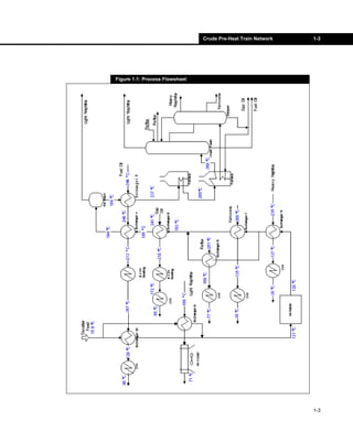
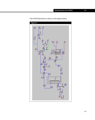
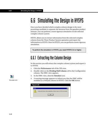
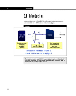
1. This tutorial presents the design of a heat exchanger network for a crude pre-heat train. The network will heat crude oil using product streams before the oil enters a desalter and pre-flash unit.
2. Process and utility streams are created, including crude oil, product streams, cooling water, and boiler feed water. Heat exchangers are added to heat the crude using the product streams.
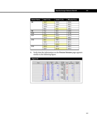
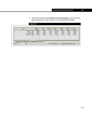
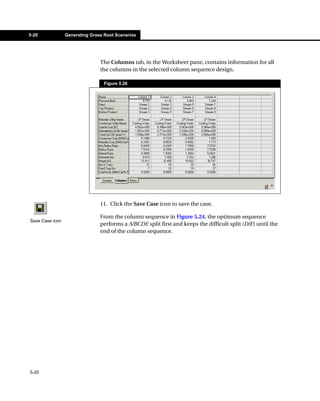
3. The worksheet is used to enter heat exchanger information and manipulate the network to complete the pre-flash section and overall heat exchanger network design.