Transport Net.pdf

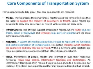
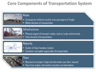
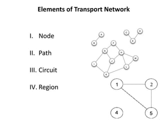
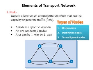
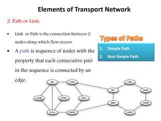
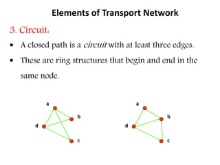
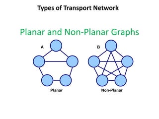
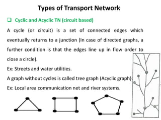
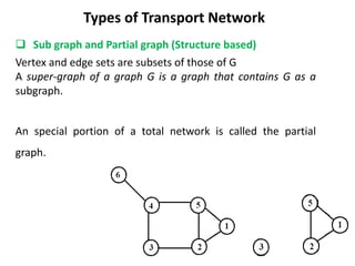
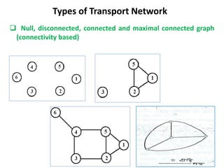
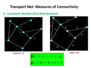
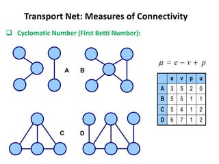
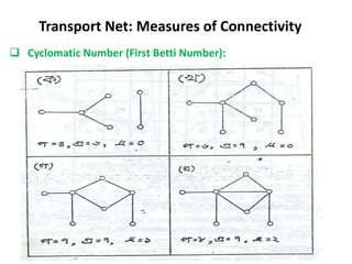
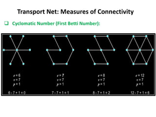
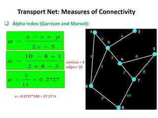
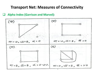
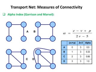
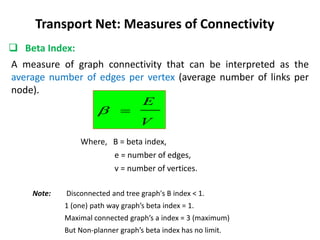
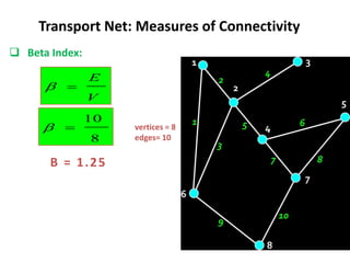
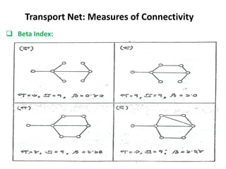
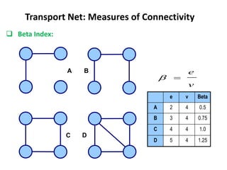
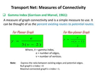
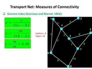
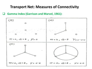
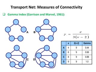
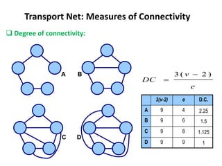
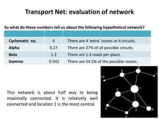
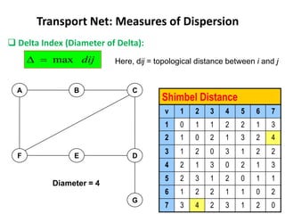
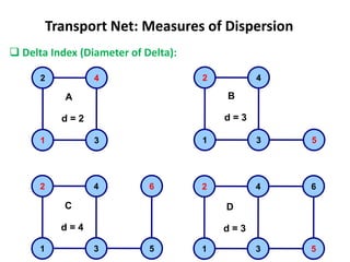
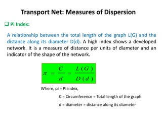
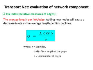
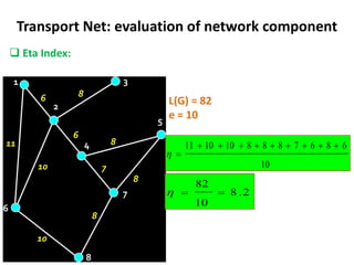
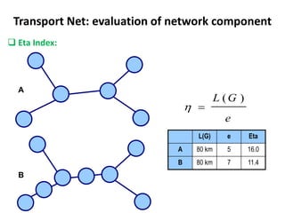
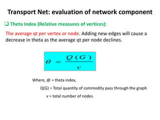
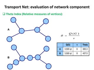
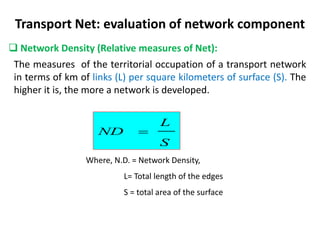
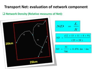
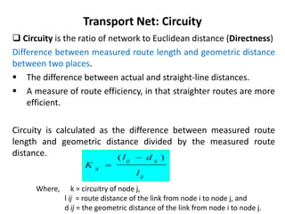
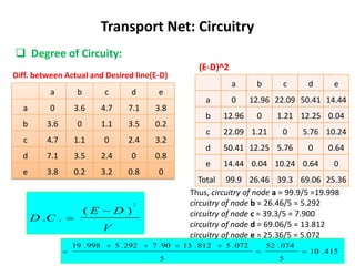
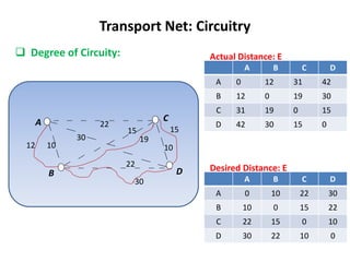
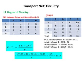
Graph theory, connectivity and accessibility, Network Analysis
Transport Network

Meaning of Transportation
 The word "TRANSPORT" has been derived from the Latin word
"TRANSPORTARE". "TRANS" means across or the other side and
"PORTARE" means carry. Transport thus means to carry to the
other side.
 the act or process of moving people or things from one place to
another
 a way of traveling from one place to another place
 a system for moving passengers or goods from one place to
another
 Transportation is the movement of people and goods over time
and space...

Core Components of Transportation System
For transportation to take place, four core components are essential:
• Modes. They represent the conveyances, mostly taking the form of vehicles that
are used to support the mobility of passengers or freight. Some modes are
designed to carry only passengers or freight, while others can carry both.
• Infrastructures. The physical support of transport modes, where routes (e.g. rail
tracks, canals or highways) and terminals (e.g. ports or airports) are the most
significant components.
• Networks. A system of linked locations that are used to represent the functional
and spatial organization of transportation. This system indicates which locations
are connected and how they are serviced. Within a network some locations are
more accessible (more connections) than others (less connections).
• Flows. Movements of people, freight and information over their respective
networks. Flows have origins, intermediary locations and destinations. An
intermediary location is often required to go from an origin to a destination. For
instance, flying from one airport to another may require a transit at hub airport.

Core Components of Transportation System

 Transportation is any means of conveying goods and people (Rashid, 1991).
 Transport or Transportation is movement of people and goods from one
location to another. Transport is performed by modes, such as air, rail, road,
water, cable, pipeline and space.
Under the form of transport location network we understand a set of
geographical local inter-connected in a system by a number of route (K.J.
Kansky, 1963) .
 “A transport network or transportation network is typically a network of
roads, streets, pipes or nearly any structure which permits either vehicular
movement of flow of some commodity (Bhaduri, 1992)”.
Transport Network

•Interconnected set of points (nodes) and lines (edges)
•Examples
-Information networks
-Social networks
-River/Stream networks
-Transportation networks
•Connectivity :
allows for analysis/problem solving
Transport Network

Network = graph
Informally a graph is a set of nodes joined by a set of lines or arrows.
•Network lines define relationships between nodes
•Flow types:
-Data
-Objects
-Materials
Transport Network
A
B G
H
F
D
C
E

•A network is made up of edges and nodes
-Edges are the “lines” of the network
-Nodes are physical locations
•Edges for all cases discussed in this module
will be roads
•Types of locations (nodes)
-Stops
-Barriers
-Facilities
-Incidents
-Origins-Destinations
Transport Network

Transport network
 Framework of routes between locations:
A permanent track (e.g. roads, rail and canals).
A scheduled service (e.g. airline, transit, train).
 Various types of links between points along which movement
can take place.
 Creates accessibility.

Transport Networks and Space
Transport Network
Space
Accessibility

Graph Representation of a Real
Network
Real Network Graph Representation

Traffic Assignment
Origin Destination
Generation Attraction
Which path?
Cost
Time
Number of connections

I. Node
II. Path
III. Circuit
IV. Region
Elements of Transport Network

1. Node:
Node is a location on a transportation route that has the
capacity to generate traffic (flow).
 A node is a specific location
 An arc connects 2 nodes
 Arcs can be 1-way or 2-way
1. Origin nodes
2. Destination nodes
3. Transshipment nodes

2. Path or Link:
 Link or Path is the connection between 2
nodes along which flow occurs.
 A path is sequence of nodes with the
property that each consecutive pair
in the sequence is connected by an
edge.
1. Simple Path
2. Non Simple Path

3. Circuit:
 A closed path is a circuit with at least three edges.
 These are ring structures that begin and end in the
same node.
a
b
c
d
a
b
c
d

Cycles and Circuits
1
2 3
4 5
6
Circuit
Cycle
Cycle

4. Region:
If any other circuit is absent in a circuit then it is
called an elementary circuit.
Space or the area in between this elementary
circuit is the region of a Transport Net.

A simple network is typically termed an undirected graph. It is “undirected”
because no information about the direction of the links has been given – just
presence or absence. Such links (without any directional information) are
also termed symmetric links.
The obvious extension of the above undirected graph is to allow for
directionality of the links – that is, a link between i and j may be from i to j (i →
j), or from j to i (j → i). Such links are termed ‘directed’ links, and the resulting
graph is a directed graph. Directed links are used to represent asymmetric
relationships between nodes.
Types of Transport Network
 Undirected and Directed TN (Direction based)
The left graph is undirected
Edges have no orientation
(default assumption)
The right graph is directed
Edges have an orientation,
e.g. edge from B to C

A Planner graph or PTN connects a two
dimensional plane at junctions, without crossing
any edges. On a street network, non-planner
graphs can model an bridge over a road.
 Planner and Non-Planner TN (Topology based)
In a Planner graph, edges only connects the nodes.
Can be drawn on a plane such that no two edges intersect.
Ex: two dimensional city road.
In a non-planner graph two or more edges can pass
through in a different elevation without touches
tehmselves.
Ex: Aieways, Overbrige etc.
cøvvbvi Rvwj
bb cøvvbvi Rvwj

Planar Non-Planar
A B
Planar and Non-Planar Graphs

A cycle (or circuit) is a set of connected edges which
eventually returns to a junction (In case of directed graphs, a
further condition is that the edges line up in flow order to
close a circle).
Ex: Streets and water utilities.
A graph without cycles is called tree graph (Acyclic graph).
Ex: Local area communication net and river systems.
 Cyclic and Acyclic TN (circuit based)

Vertex and edge sets are subsets of those of G
A super-graph of a graph G is a graph that contains G as a
subgraph.
An special portion of a total network is called the partial
graph.
 Sub graph and Partial graph (Structure based)

 Null, disconnected, connected and maximal connected graph
(connectivity based)

 Physical, fictional and service net (function based)
1. Physical Net:
When a number of edges and nodes are interconnected to create
integrated communication system which has a physical existence in
the real world then it is called physical transport network.
Ex: Road, Rail way.
2. Functional Net:
It has no visible track and identified spatial pattern like as physical net.
But modes of transport generally moves through a defined way. This
kind of transport net is called Functional net.
Ex: Ocean and air ways net.
3. Service Net:
If transportation modes moves through a partial way of the large physical
net then it is called as service net.

 According to Speight 1978 (Morphology Based)
 Rectangular Net:
If two path/edges are intersect with 90 degree angle, then the physical net stretch
in a rectangular shape. Ex: Roman city, USA, Chandigarh (India) and Upashahar
housing state in BD.
 Reflected net:
If many edges spread from a origin point or node then it is known as reflected net.
Ex: Physical net of the primate city.
 Tree shape net:
If a transport net spread like as the branches of tree, but can not create any circuit
then it is called tree shape net. Ex: National railway of AUS.
 Corridor net:
If huge traffic and goods flow in the specified track in two defined space then that
important track is known as coeditor net.

Graph Theory: Indexes and Measures

Connectivity: the relative degree of connectedness within a
transportation network.
High connectivity = low isolation, high accessibility.
Low connectivity = high isolation, low accessibility.
Connectivity is a measure of accessibility without regard to
distance.
Places with high connectivity are often considered important
since they are the best connected.
Connectivity of T.N.

First must reduce the transportation network to a matrix consisting
of ones (1) and zeros (0).
If two locations (vertices) are directly connected by a link (edge),
code with a 1.
If two locations(vertices) are not directly connected by a link(edge),
code with a 0.
Connectivity Matrix

Connectivity is based on topologic distance.
Topological distance – the number of direct connections or steps
separating two nodes.
Transposing the matrix is done to account for flow in both directions.
A---B and B---A
Both of these have a topological distance of 1.
Connectivity Matrix

Konig Number system: According to GERMAN Mathematician DENES KONIG(1936)
The König number (or associated number) is the number of edges from any node in
a network to the furthest node from it. This is a topological measure of distance, in
edges rather than in kilometers. A low associated number indicates a high degree of
connectivity; the lower the König number, the greater the Centrality of that node.
Connectivity Matrix
Application of Konig number to measure centrality of a transport net
A
B
C D
E
F
G

Connectivity Matrix
A
B
C
D
E
V
V
A B C D E Total
A 0 1 1 1 2 5
B 1 0 2 2 3 8
C 1 2 0 2 3 8
D 1 2 2 0 1 6
E 2 3 3 1 0 9
Measurements of Accessibility:
Hence, inter node-edge no. of A is the lowest, So the accessibility
and centrality is the highest in this node.
Or A is the central place of this network.

Transport Net: Measures of Connectivity
 Cyclomatic Number (First Betti Number):
An index that is the difference between the number of edges and
vertices.
Where, μ = cyclomatic number,
e = number of edges,
v = number of vertices, and
p = number of subgraphs.
Note: in most cases p = 1.
p
v
e 


μ

Vertices = 8 Edges =10
p
v
e 


μ
3
1
8
10
μ 




e v p u
A 3 5 2 0
B 5 5 1 1
C 5 4 1 2
D 6 7 1 2
A B
C D
p
v
e 




A measure of graph connectivity that can be interpreted as the
ratio of existing circuits to the maximum possible circuits.
 Alpha Index (Garrison and Marvel):
5
2 



v
p
v
e
 )
1
(
2
)
1
(






V
v
v
p
v
e

For Planner Graph For Non-planner Graph
Where, a = alpha index,
v = number of vertices, and
p = number of subgraphs.
Note: a index generally expressed by percentage(%).
The higher the index value, the higher the connectivity.
Maximal connected graph’s a index = 1.

vertices = 8
edges= 10
5
2 



v
p
v
e

5
8
2
1
8
10






2727
.
0
11
3



a = 0.2727*100 = 27.27 %

A B
C D
(e-v+p) 2v-5 Alpha
A 0 3 0.0
B 1 3 0.33
C 2 3 0.66
D 3 3 1.0
5
2 



v
p
v
e


A measure of graph connectivity that can be interpreted as the
average number of edges per vertex (average number of links per
node).
 Beta Index:
V
E


Where, B = beta index,
v = number of vertices.
Note: Disconnected and tree graph's B index < 1.
1 (one) path way graph’s beta index = 1.
Maximal connected graph’s a index = 3 (maximum)
But Non-planner graph’s beta index has no limit.

 Beta Index:
V
E


vertices = 8
edges= 10
8
10


B = 1.25

 Beta Index:

A B
C D
e v Beta
A 2 4 0.5
B 3 4 0.75
C 4 4 1.0
D 5 4 1.25
v
e


 Beta Index:

)
2
(
3 

v
e

 Gamma Index (Garrison and Marvel, 1961):
A measure of graph connectivity and is a simple measure to use. It
can be thought of as the percent existing routes to potential routes.
2
)
1
( 

v
v
e

Where, V = gamma index,
Note: Express the ratio between existing edges and potential edges.
Null graph’s v index = 0
Maximal connected graph’s v index = 1.

vertices = 8
edges= 10
)
2
(
3 

v
e

)
2
8
(
3
10



56
.
0
18
10




A B
C D
e 3(v-2) Gamma
A 4 9 0.44
B 6 9 0.66
C 8 9 0.88
D 9 9 1.0
 
2
3 

v
e


 Degree of connectivity:
It describes the transport net as a unit component. It express each
and every net by the percentage value (%). It can compare the
other indices of connectivity measurement.
e
v
v
c
d
/
2
)
1
(
.
.


e
v
c
d
)
2
(
3
.
.


Where, d.c. = degree of connectivity,

A B
C D
3(v-2) e D.C.
A 9 4 2.25
B 9 6 1.5
C 9 8 1.125
D 9 9 1
e
v
DC
)
2
(
3 

 Degree of connectivity:

Transport Net: evaluation of network
So what do these numbers tell us about the following hypothetical network?
Cyclomatic no. 4 There are 4 ‘extra’ routes or 4 circuits.
Alpha 0.27 There are 27% of all possible circuits.
Beta 1.3 There are 1.3 roads per place.
Gamma 0.542 There are 54.2% of the possible routes.
This network is about half way to being
maximally connected. It is relatively well
connected and location 1 is the most central.

Shimbel Distance
v 1 2 3 4 5 6 7
1 0 1 1 2 2 1 3
2 1 0 2 1 3 2 4
3 1 2 0 3 1 2 2
4 2 1 3 0 2 1 3
5 2 3 1 2 0 1 1
6 1 2 2 1 1 0 2
7 3 4 2 3 1 2 0
F
A
E
B
D
C
G
Diameter = 4
 Delta Index (Diameter of Delta):
Transport Net: Measures of Dispersion
Here, dij = topological distance between i and j
dij
max



1
2
3
4
1
2
3
4
5
1
2
3
4
5
6
1
2
3
4
5
6
A
d = 2
B
d = 3
C
d = 4
D
d = 3
 Delta Index (Diameter of Delta):

 Pi Index:
A relationship between the total length of the graph L(G) and the
distance along its diameter D(d). A high index shows a developed
network. It is a measure of distance per units of diameter and an
indicator of the shape of the network.
)
(
)
(
d
D
G
L
d
C



Where, pi = Pi index,
C = Circumference = Total length of the graph
d = diameter = distance along its diameter

Pi Index and the Shape of Transportation Networks
d
Highly developed
(High Pi) Least
developed
(Low
Pi)
 Pi Index:
)
(
)
(
d
D
G
L



L(G) = 82
D(d) = 35
8
6
11
10
6
8
6
7
8
8
8
10
10
11














342
.
2
35
82



 Pi Index:

 Detour Index (Relative measures of Distance):
A measure of the efficiency of a network in terms of how well it overcomes
distance or the friction of distance. The closer the detour index gets to 1, the
more the network is spatially efficient. Networks having a detour index of 1 are
rarely, if ever, seen and most networks would fit on an asymptotic curve getting
close to 1, but never reaching it.
The straight distance (DD) between two nodes may be 40 km but the transport
distance (TD; real distance) is 50 km. The detour index is thus 0.8 (40 / 50).
TD
DD
I
D 
.
.
Where, D.I. = Detour index,
DD = Direct or straight Distance
TD = Transport Distance

Transport Distance (TD) Straight Distance (DD)
TD
DD
I
D 
.
.
91
.
0
53
48
9
8
11
13
12
9
8
10
11
10
.
. 










I
D
 Detour Index (Relative measures of Distance):

The average length per link/edge. Adding new nodes will cause a
decrease in eta as the average length per link declines.
Transport Net: evaluation of network component
 Eta Index (Relative measures of edges):
e
G
L )
(


Where, n = Eta index,
L (G) = Total length of the graph
e = total number of edges

 Eta Index:
L(G) = 82
e = 10
10
6
8
6
7
8
8
8
10
10
11 










2
.
8
10
82




L(G) e Eta
A 80 km 5 16.0
B 80 km 7 11.4
A
B
e
G
L )
(


 Eta Index:

 Theta Index (Relative measures of vertices):
The average qt per vertex or node. Adding new edges will cause a
decrease in theta as the average qt per node declines.
v
G
Q )
(


Where, @ = theta index,
Q(G) = Total quantity of commodity pass through the graph
v = total number of nodes

v
G
Q )
(


Q(G) v Theta
A 3,500 qt 6 583.3
B 3,500 qt 8 437.5
A
B
 Theta Index (Relative measures of vertices):

 Network Density (Relative measures of Net):
The measures of the territorial occupation of a transport network
in terms of km of links (L) per square kilometers of surface (S). The
higher it is, the more a network is developed.
S
L
ND 
Where, N.D. = Network Density,
L= Total length of the edges
S = total area of the surface

 Network Density (Relative measures of Net):
S
L
ND 
)
28
25
(
)
9
8
11
13
12
(






ND
2
/
076
.
0
700
53
km
km
ND 


 Circuity is the ratio of network to Euclidean distance (Directness)
Difference between measured route length and geometric distance
between two places.
 The difference between actual and straight-line distances.
 A measure of route efficiency, in that straighter routes are more
efficient.
Circuity is calculated as the difference between measured route
length and geometric distance divided by the measured route
distance.
Transport Net: Circuity
Where, k = circuitry of node j,
l ij = route distance of the link from node i to node j, and
d ij = the geometric distance of the link from node i to node j.
ij
ij
ij
ij
l
d
l
K
)
( 


 Circuity:
ij
ij
ij
ij
l
d
l
K
)
( 

6
.
13
)
10
6
.
13
( 

ij
K
265
.
0

ij
K
 A value of 0 means the route is non-circuitous (straight).
 A value approaching 1 means the route is very circuitous.
Values will never reach 1, since the potential difference between actual distance
and geometric distance is infinite.
Circuitry ranges from 0 to 1.

 Degree of Circuity:
A node based measurement of the actual versus geometric distance
summed from one node to all other nodes along the shortest route.
V
D
E
C
D
)
(
.
.
2


Where, D.C. = Degree of Circuitry,
E = Existing Route.
D = Desired Line
V = Vertices.

Transport Net: Circuitry
 Degree of Circuitry:

a b c d e
a 0 13.6 23.7 37.1 23.8
b 13.6 0 10.1 23.5 10.2
c 23.7 10.1 0 13.4 25.2
d 37.1 23.5 13.4 0 11.8
e 23.8 10.2 25.2 11.8 0
Actual Distance: E
a b c d e
a 0 10 19 30 20
b 10 0 9 20 10
c 19 9 0 11 22
d 30 20 11 0 11
e 20 10 22 11 0
Desired Distance: E

a b c d e
a 0 3.6 4.7 7.1 3.8
b 3.6 0 1.1 3.5 0.2
c 4.7 1.1 0 2.4 3.2
d 7.1 3.5 2.4 0 0.8
e 3.8 0.2 3.2 0.8 0
a b c d e
a 0 12.96 22.09 50.41 14.44
b 12.96 0 1.21 12.25 0.04
c 22.09 1.21 0 5.76 10.24
d 50.41 12.25 5.76 0 0.64
e 14.44 0.04 10.24 0.64 0
Total 99.9 26.46 39.3 69.06 25.36
(E-D)^2
Diff. between Actual and Desired line(E-D)
V
D
E
C
D
)
(
.
.
2


415
.
10
5
074
.
52
5
072
.
5
812
.
13
90
.
7
292
.
5
998
.
19







Thus, circuitry of node a = 99.9/5 =19.998
circuitry of node b = 26.46/5 = 5.292
circuitry of node c = 39.3/5 = 7.900
circuitry of node d = 69.06/5 = 13.812
circuitry of node e = 25.36/5 = 5.072

A B C D
A 0 12 31 42
B 12 0 19 30
C 31 19 0 15
D 42 30 15 0
Actual Distance: E
A B C D
A 0 10 22 30
B 10 0 15 22
C 22 15 0 10
D 30 22 10 0
Desired Distance: E
C
D
A
B
22
15
10
19
15
30
30
22
10
12

(E-D)^2
Diff. between Actual and Desired line(E-D)
A B C D
A 0 2 9 12
B 2 0 4 8
C 9 4 0 5
D 12 8 5 0
A B C D
A 0 4 81 144
B 4 0 16 64
C 81 16 0 25
D 144 64 25 0
Total 229 84 122 233
V
D
E
C
D
)
(
.
.
2


75
.
41
4
167
4
25
.
58
50
.
30
21
25
.
57






Thus, circuitry of node A = 229/4 = 57.25
circuitry of node B = 84/4 = 21
circuitry of node C = 122/4 = 30.50
circuitry of node D = 233/4 = 58.25

Refrences
Idous and Wilson, 2000. Graph and Applications: An Introductory Approach,
Springer, 2000.
Wasserman and Faust, 2008. Social Network Analysis, Cambridge University
Press, London.
Geoffrey, S. and Monsen, K. E., 2008. Network Analysis, ISSN 0085-7130 © Telenor
ASA 2008, Norway.
i“gx, •m.i. Av. Ges Ab¨vb¨ (2007), ÒcwienY f~‡Mvj: D‡Ïk¨ I ¸i“Z¡Ó, mye©Y Rqš—x: ¯§viK
msKjb, 2007, c„. 47-87.
Zvnv, Avey (2002). ÒAvKvka„Z f~wPÎ I cwienY †bUIqvK© we‡klYÓ, cvV¨cy¯—K cÖKvkbv †evW©, ivRkvnx
wek¦we`¨vjq, c„. 61-87.

C
D
B
22
15
10
19
15
30
30
22
10
A
12
B
C
D
E
8
13
10
12
20
18
17
22
9
6

Transport Net.pdf

More Related Content

What's hot

Similar to Transport Net.pdf

Recently uploaded

Transport Net.pdf