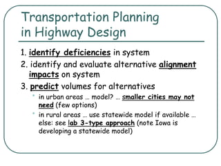
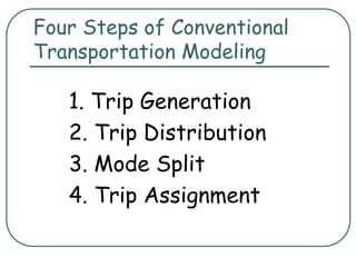
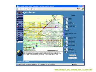
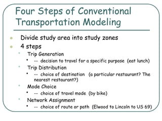
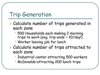
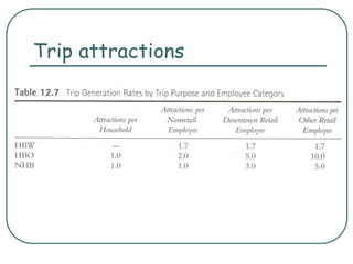
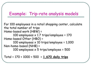
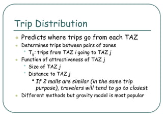
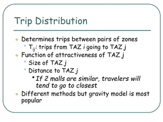
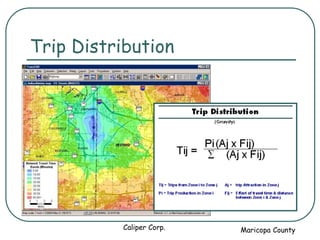
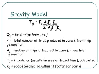
This document discusses transportation planning and traffic estimation. It covers the key components of transportation planning including identifying deficiencies in transportation systems, evaluating alternative transportation alignments, and predicting traffic volumes. The four steps of transportation demand modeling are also outlined: trip generation, trip distribution, mode choice, and traffic assignment. Transportation planning involves collecting travel data, identifying current and future transportation needs, and developing solutions to meet travel demand. The results of transportation planning and modeling are used in highway design projects.

1. Transportation Planning
and Traffic Estimation
CE 453 Lecture 5

2. Objectives
1. Identify highway system components
2. Define transportation planning
3. Recall the transportation planning process
and its design purposes
4. Identify the four steps of transportation
demand modeling and describe modeling
basics.
5. Explain how transportation planning and
modeling process results are used in highway
design.

3. Highway System Components
1. Vehicle
2. Driver (and peds./bikes)
3. Roadway
4. Consider characteristics, capabilities, and
interrelationships in design
Start with demand needs (number of lanes?)

4. Transportation Planning
(one definition)
Activities that:
1. Collect information on performance
2. Identify existing and forecast future
system performance levels
3. Identify solutions
Focus: meet existing and forecast travel
demand

5. Where does planning fit in?

6. Transportation Planning
in Highway Design
1. identify deficiencies in system
2. identify and evaluate alternative alignment
impacts on system
3. predict volumes for alternatives
• in urban areas … model? … smaller cities may not
need (few options)
• in rural areas … use statewide model if available …
else: see lab 3-type approach (note Iowa is
developing a statewide model)

10. Truck Traffic

12. Planning at 3 levels
 State … STIP Statewide
Transportation Improvement Program
(list of projects)
 Regional … MPO Metropolitan Planning
Organization (>50,000 pop.), 25 year
long range plan and TIP (states now
also do LRP)
 Local …project identification and
prioritization

13. Four Steps of Conventional
Transportation Modeling
1. Trip Generation
2. Trip Distribution
3. Mode Split
4. Trip Assignment

14. Study Area
 Clearly define the area under consideration
• Where does one entity end?
• May be defined by county boundaries, jurisdiction,
town centers

15. Study Area
 May be regional
 Metropolitan area – Des Moines including
suburbs, Ankeny, etc.
• Overall impact to major street/highway network
 Local – e.g., impact of trips to new Ames mall
• Impact on local street/highway system
• Impact on intersections
• Need for turning lane or new signal – can a model do
this level of detail?

16. Study Area
 Links and nodes
 Simple representation of the geometry of
the transportation systems (usually major
roads or transportation routes)
 Links: sections of roadway (or railway)
 Nodes: intersection of 2+ links
 Centroids: center of TAZs
 Centroid connectors: centroid to roadway
network where trips load onto the network

17. Travel Analysis Zones (TAZs)
 Homogenous urban activities (generate same
types of trips)
•Residential
•Commercial
•Industrial
 May be as small as one city block or as large as
10 sq. miles
 Natural boundaries --- major roads, rivers,
airport boundaries
 Sized so only 10-15% of trips are intrazonal

18. www.sanbag.ca.gov/ planning/subr_ctp_taz.html

19. Four Steps of Conventional
Transportation Modeling
 Divide study area into study zones
 4 steps
• Trip Generation
• -- decision to travel for a specific purpose (eat lunch)
• Trip Distribution
• -- choice of destination (a particular restaurant? The
nearest restaurant?)
• Mode Choice
• -- choice of travel mode (by bike)
• Network Assignment
• -- choice of route or path (Elwood to Lincoln to US 69)

20. Trip
Generation
Model Step #1…

21. Trip Generation
 Calculate number of trips generated in
each zone
• 500 Households each making 2 morning
trips to work (avg. trip ends ~ 10/day!)
• Worker leaving job for lunch
 Calculate number of trips attracted to
each zone
• Industrial center attracting 500 workers
• McDonalds attracting 200 lunch trips

22. Trip Generation
 Number of trips that begin from or
end in each TAZ
 Trips for a “typical” day
 Trips are produced or attracted
 # of trips is a function of:
• TAZs land use activities
• Socioeconomic characteristics of TAZ
population

23. Trip Generation
ModelManager 2000™
Caliper Corp.

24. Trip Generation
 3 variables related to the factors that influence trip
production and attraction (measurable variables)
• Density of land use affects production & attraction
• Number of dwellings, employees, etc. per unit of land
• Higher density usually = more trips
• Social and socioeconomic characters of users influence
production
• Average family income
• Education
• Car ownership
• Location
• Traffic congestion
• Environmental conditions

25. Trip Generation
 Trip purpose
• Zonal trip making estimated separately by trip
purpose
• School trips
• Work trips
• Shopping trips
• Recreational trips
• Travel behavior depends on trip purpose
• School & work trips are regular (time of day)
• Recreational trips highly irregular

26. Trip Generation
 Forecast # of trips that produced or attracted by
each TAZ for a “typical” day
 Usually focuses on Monday - Friday
 # of trips is forecast as a function of other variables
 Attraction
• Number and types of retail facilities
• Number of employees
• Land use
 Production
• Car ownership
• Income
• Population (employment characteristics)

27. Trip Purpose
 Trips are estimated by purpose (categories)
• Work
• School
• Shopping
• Social or recreational
• Others (medical)
 Travel behavior of trip-makers depends somewhat on trip purpose
• Work trips
• regular
• Often during peak periods
• Usually same origin/destination
• School trips
• Regular
• Same origin/destination
• Shopping recreational
• Highly variable by origin and destination, number, and time of
day

28. Household Based
 Trips based on “households” rather than individual
 Individual too complex
 Theory assumes households with similar characteristics
have similar trip making characteristics
 However
• Concept of what constitutes a “household” (i.e. 2-parent
family, kids, hamster) has changed dramatically
• Domestic partnerships
• Extended family arrangements
• Single parents
• Singles
• roommates

29. Trip Generation Analysis
 3 techniques
• Cross-classification
• Covered in 355
• Multiple regression analysis
• Mathematical equation that describes trips as a
function of another variable
• Similar in theory to trip rate
• Won’t go into
• Trip-rate analysis models
• Average trip-production or trip-attraction rates for
specific types of producers and attractors
• More suited to trip attractions

30. Trip attractions

31. Example: Trip-rate analysis models
For 100 employees in a retail shopping center, calculate
the total number of trips
Home-based work (HBW) =
100 employees x 1.7 trips/employee = 170
Home-based Other (HBO) =
100 employees x 10 trips/employee = 1,000
Non-home-based (NHB) =
100 employees x 5 trips/employee = 500
Total = 170 + 1000 + 500 = 1,670 daily trips

32. Trip
Distribution
Model Step #2…

33. Trip Distribution
 Predicts where trips go from each TAZ
 Determines trips between pairs of zones
• Tij: trips from TAZ i going to TAZ j
 Function of attractiveness of TAZ j
• Size of TAZ j
• Distance to TAZ j
•If 2 malls are similar (in the same trip
purpose), travelers will tend to go to closest
 Different methods but gravity model is most popular

34. Trip Distribution
 Determines trips between pairs of zones
• Tij: trips from TAZ i going to TAZ j
 Function of attractiveness of TAZ j
• Size of TAZ j
• Distance to TAZ j
•If 2 malls are similar, travelers will
tend to go to closest
 Different methods but gravity model is most
popular

35. Trip Distribution
Maricopa County
Caliper Corp.

36. Gravity Model
Tij = Pi AjFijKij
Σ AjFijKij
Qij = total trips from i to j
Pi = total number of trips produced in zone i, from trip
generation
Aj = number of trips attracted to zone j, from trip
generation
Fij = impedance (usually inverse of travel time), calculated
Kij = socioeconomic adjustment factor for pair ij

37. Mode Choice
Model Step #3…

38. Mode Choice
 In most situations, a traveler has a
choice of modes
• Transit, walk, bike, carpool, motorcycle,
drive alone
 Mode choice/mode split determines #
of trips between zones made by auto
or other mode, usually transit

39. 39
Characteristics Influencing
Mode Choice
 Availability of parking
 Income
 Availability of transit
 Auto ownership
 Type of trip
• Work trip more likely transit
• Special trip – trip to airport or baseball stadium served
by transit
• Shopping, recreational trips by auto
 Stage in life
• Old and young are more likely to be transit dependent

40. 40
Characteristics Influencing
Mode Choice
 Cost
• Parking costs, gas prices, maintenance?
• Transit fare
 Safety
 Time
• Transit usually more time consuming (not in NYC or DC
…)
 Image
• In some areas perception is that only poor ride transit
• In others (NY) everyone rides transit

41. Mode Choice Modeling
 A numerical method to describe how
people choose among competing
alternatives (don’t confuse model and
modal)
 Highly dependent on characteristics
of region
 Model may be separated by trip
purposes

42. Utility and Disutility Functions
 Utility function: measures satisfaction derived
from choices
 Disutility function: represents generalized costs
of each choice
 Usually expressed as the linear weighted sum of
the independent variables of their
transformation
U = a0 + a1X1 + a2X2 + ….. + arXr
U: utility derived from choice
Xr: attributes
ar: model parameters

43. Logit Models
 Calculates the probability of selecting
a particular mode
p(K) = ____eUk__
 eUk
p: probability of selecting mode k

44. Logit Model Example 1
Utility functions for auto and transit
U = ak– 0.35t1 – 0.08t2 – 0.005c
ak = mode specific variable
t1 = total travel time (minutes)
t2 = waiting time (minutes)
c = cost (cents)
Do you agree with
the relative
magnitude of the
time parameters? Is
there double
counting/colinearity?

45. Logit Model Example 1 (cont)
Travel characteristics between two zones
Uauto = -0.46 – 0.35(20) – 0.08(8) – 0.005(320) = -9.70
Utransit = -0.07 – 0.35(30) – 0.08(6) – 0.005(100) = -11.55
Variable Auto Transit
ak -0.46 -0.07
t 1 20 30
t 2 8 6
c 320 100
Do you agree with
the relative
magnitude of the
mode specific
parameters? How
much effect does
cost have?

46. Logit Model Example 1 (cont)
Uauto = -9.70
Utransit = -11.55
Logit Model:
p(auto) = ___eUa __ = _____e-9.70 ____ = 0.86
eUa + eUt e-9.70 + e-11.55
p(transit) = ___eUt __ = _____e-11.55 ____ = 0.14
eUa + eUt e-9.70 + e-11.55

47. Logit Model Example 2
The city decides to spend money to create and improve
bike trails so that biking becomes a viable option, what
percent of the trips will be by bike?
Assume:
• A bike trip is similar to a transit trip
• A bike trip takes 5 minutes more than a transit trip but
with no waiting time
• After the initial purchase of the bike, the trip is “free”

48. Travel characteristics between two zones
Uauto = -0.46 – 0.35(20) – 0.08(8) – 0.005(320) = -9.70
Utransit = -0.07 – 0.35(30) – 0.08(6) – 0.005(100) = -11.55
Ubike = -0.07 – 0.35(35) – 0.08(0) – 0.005(0) = -12.32
Variable Auto Transit Bike
ak -0.46 -0.07 -0.07
t 1 20 30 35
t 2 8 6 0
c 320 100 0
Logit Model Example 2 (cont)

49. Uauto = -9.70, Utransit = -11.55, Ubike = -12.32
Logit Model:
p(auto) = _____eUa ____ = _______e-9.70 ______ = 0.81
eUa + eUt +eUb e-9.70 + e-11.55 + e-12.32
p(transit) = _____eUt__ __ = ______e-11.55 ______ = 0.13
eUa + eUt +eUb e-9.70 + e-11.55 + e-12.32
p(bike) = _____eUt__ __ = ________e-11.55 ______ = 0.06
eUa + eUt +eUb e-9.70 + e-11.55 + e-12.32
Notice that auto
lost share even
though its “utility”
stayed the same
Logit Model Example 2 (cont)

50. Traffic Assignment
(Route Choice)
Caliper Corp.
Model Step #4…

51. Trip Assignment
 Trip makers choice of path between
origin and destination
 Path: streets selected
 Transit: usually set by route
 Results in estimate of traffic volumes
on each roadway in the network

52. Person Trips vs. Vehicle Trips
 Trip generation step calculated total
person trips
 Trip assignment deals with volume not
person trips
 Need to adjust person trips to reflect
vehicle trips
 Understand units during trip generation
phase

53. Person Trips vs. Vehicle Trips
Example
Usually adjust by average auto occupancy
Example:
If:
 average auto occupancy = 1.2
 number of person trips from zone 1 = 550
So:
Vehicle trips = 550 person trips/1.2 persons per vehicle =
458.33 vehicle trips

54. Time of Day Patterns
 Trip generation usually based on 24-
hour period
 LOS calculations usually based on
hourly time period
 Hour, particularly peak, is often of
more interest than daily

55. Time of Day Patterns
 Common time periods
• Morning peak
• Afternoon peak
• Off-peak
 Calculation of trips by time of day
• Use of factors (e.g., morning peak may be
11% of daily traffic)
• Estimate trip generation by hour

56. Minimum Path
 Theory: users will select the quickest
route between any origin and destination
 Several route choice models (all based on
some “minimum” path)
• All or nothing
• Multipath
• Capacity restraint

57. Minimum Tree
 Starts at zone and selects minimum path to
each successive set of nodes
 Until it reaches destination node
1
2
3
4
5
(3)
(4)
(2)
(4)
(7)
Path from 1 to 5

58. Minimum Tree
1
2
3
4
5
(3)
(4)
(2)
(4)
(7)
1. Path from 1 to 5 first passes thru 4
2. First select minimum path from 1 to 4
3. Path 1-2-4 has impedance of 5
4. Path 1-3-4 has impedance of 8
5. Select 1-2-4
See CE451/551
notes for more on
shortest path
computations –
several methods are
available

59. All or Nothing
 Allocates all volume between zones to
minimum path based on free-flow link
impedances
 Does not update as the network loads
 Becomes unreliable as volumes and
travel time increases

60. Multi-Path
 Assumes that all traffic will not use shortest path
 Assumes that traffic will allocate itself to
alternative paths between a pair of nodes based on
costs
 Uses some method to allocate percentage of trips
based on cost
• Utility functions (logit)
• Or some other relationship based on cost
 As cost increases, probability that the route will
be chosen decreases

61. Capacity Restraint
 Once vehicles begin selecting the
minimum path between a set of nodes,
volume increase and so do travel
times
 Original minimum paths may no longer
be the minimum path
 Capacity restraint assigns traffic
iteratively, updating impedance at
each step

62. Sizing
Facilities

63. Sizing
Facilities

64. Sizing
Facilities