This paper analyzes the transient stability of the IEEE 9 Bus system using Power World Simulator, focusing on the stability post-disturbances caused by faults and load changes. It employs both the Runga and Euler methods to evaluate system performance under three-phase balanced faults, noting that Runga method provides faster responses compared to Euler method. The results highlight the importance of maintaining low critical clearing times to preserve system synchronism and stability.

1. Ramandeep Kaur Int. Journal of Engineering Research and Applications www.ijera.com
ISSN: 2248-9622, Vol. 6, Issue 1, (Part - 2) January 2016, pp.35-39
www.ijera.com 35|P a g e
Transient Stability Analysis of IEEE 9 Bus System in Power
World Simulator
Ramandeep Kaur, Er. Divesh Kumar
Department of Electrical Engineering Bhai Gurdas Institue of Engineering and Technology Sangrur, India
Department of Electrical Engineering Bhai Gurdas Institute of Engineering and Technology Sangrur, India
ABSTRACT
It is widely accepted that transient stability is an important aspect in designing and upgrading electric power
system.
The objective of this paper was to investigate and understand the stability of power system
In this paper, modelling and transient stability analysis of IEEE 9 bus system was performed using POWER
WORLD SIMULATOR. The load flow studies were performed to determine pre-fault conditions in the system
using Newton-Raphson method. With the help of three-phase balanced fault, the variations in power angle and
frequency of the system were studied. Frequency is a reliable indicator if deficiency condition in the power
systems exists or not. For three-phase balanced fault, fast fault clearing time was analysed to bring back the
system to the stability. Further, comparison between Runga method and Euler method for better results was
performed. Hence, impact of load switching on system was also computed so as to bring system to steady state.
Keywords: power system stability, clearing time, transient stability, load switching, three-phase balanced fault,
steady state.
I. INTRODUCTION
Now-a-days, it has become a necessity to
maintain synchronism because the system is
expanding day-by-day and these results in installation
of larger machines. Due to this, transient
disturbances are increasing continuously in power
system. The transient disturbances are caused by the
changes in the load, switching operations, faults and
loss excitations. Thus, it is very important to regain
synchronism or equilibrium after disturbances in the
electrical utilities. Hence, thorough analysis of
transient stability is required to reduce problems such
as blackouts, loss of synchronism, etc.
The term stability refers to maintenance of
synchronism and stability limit refers to maximum
power flow possible in the system or a part of system
at which system is operating with stability. Power
system stability is the property of power System that
enables it to remains in a state of equilibrium under
normal operating conditions an to regain equilibrium
after being subjected to disturbances.
Power system stability can be broadly grouped
into steady state stability, transient stability and
dynamic stability. Steady state stability is the
capability of an electric power system to maintain
synchronism between machines when small slow
disturbance occurs. Dynamic stability is the ability of
a power system to remain in synchronism after the
initial swing until the system has settled down to the
new steady state equilibrium conditions.
In this paper, the main emphasis is given to transient
stability of system. Transient stability is the ability of
system to remain in synchronism during the period of
disturbance and prior to the time that the governors
can act. The transient stability analysis is carried out
for a short time period that will be equal to the time
of one swing. This analysis is carried out to
determine whether the system losses stability during
the first swing or not.
Transient stability depends on both initial
operating state of system and state when disturbance
occurs. The disturbance alters the system such that
the post disturbance steady state operation will be
different from that prior to the disturbance. Instability
is in the form of aperiodic drift due to insufficient
synchronizing torque, and is referred to as first swing
stability.
In this paper, Transient stability analysis is
performed with the help of three-phase balanced
fault. A fault which gives rise to equal fault currents
in the lines with 120 degree displacement is known as
three phase fault or symmetrical fault.
Faults could happen when a phase establishes a
connection with another phase, lightning, insulation
deterioration, wind damage, trees falling across lines,
etc.
To analyse swing behaviour of system it is
solved by two methods i.e. Runga method and Euler
method. Swing equation is the electromechanical
equation describ-ingrelative motion of the rotor load
angle (δ) with respect to the stator field as a function
of time is known as Swing equation. In most
disturbances, linearization is not per-missible and the
RESEARCH ARTICLE OPEN ACCESS

2. Ramandeep Kaur Int. Journal of Engineering Research and Applications www.ijera.com
ISSN: 2248-9622, Vol. 6, Issue 1, (Part - 2) January 2016, pp.35-39
www.ijera.com 36|P a g e
nonlinear swing equation must be solved because
oscillations are of such magnitude.
Power flow analysis is called the backbone of
power system analysis. Power system fault analysis is
one of the basic problems in power system
engineering.
The single line diagram of IEEE 9 bus model is
shown in figure1:
Figure1: IEEE 9 BUS MODEL in power world
simulator
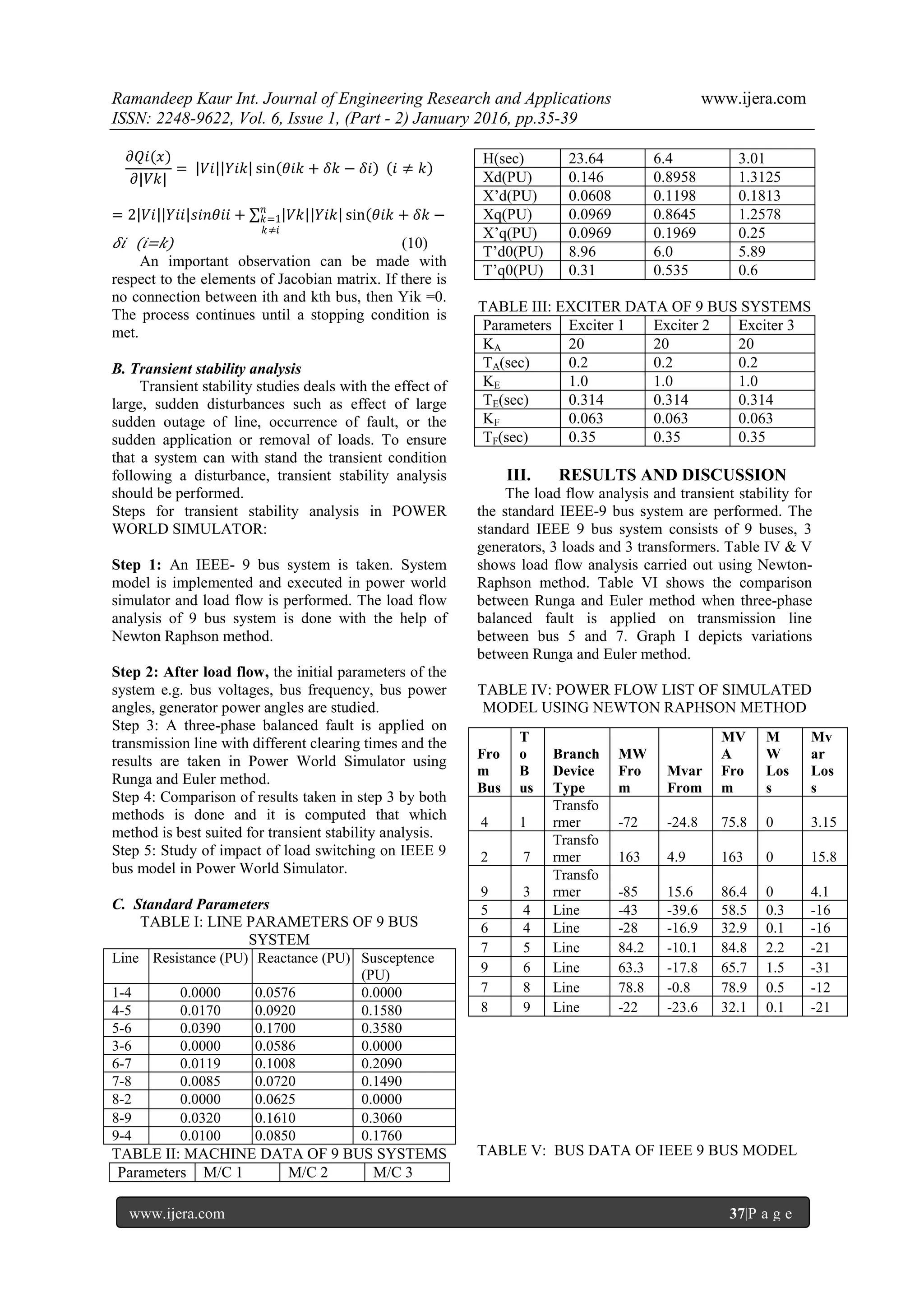
II. PROBLEM FORMULATION
A. Power Flow Studies
In transient stability studies, it is necessary to
have the knowledge of pre-fault voltages magnitudes.
The main information obtained from the power flow
study comprises of magnitudes and phase angles of
bus voltages, real and reactive powers on
transmission lines, real and reactive powers at
generator buses, other variables being specified. The
pre-fault conditions can be obtained from results of
load flow studies by the Newton-Raphson iteration
method.
The Newton-Raphson method is the practical
method of load flow solution of large power
networks. Convergence is not affected by the choice
of slack bus. This method begins with initial guesses
of all unknown variables such as voltage magnitude
and angles at load buses and voltage angles at
generator buses. Next, a Taylor Series is written, with
the higher order terms ignored, for each of the power
balance equations included in the system of
equations.
We first consider the presence of PQ buses only apart
from a slack bus.
For an ith bus,
Pi = 𝑉𝑖 𝑉𝑘 |𝑌𝑖𝑘|cos⁡(𝜃𝑖𝑘 + 𝛿𝑘 −𝑛
𝑘=1 𝛿𝑖) =
𝑃𝑖( 𝑉 , 𝛿) (1)
Qi = 𝑉𝑖 𝑉𝑘 |𝑌𝑖𝑘|sin⁡(𝜃𝑖𝑘 + 𝛿𝑘 −𝑛
𝑘=1 𝛿𝑖) =
𝑄𝑖( 𝑉 , 𝛿) (2)
i.e., both real and reactive powers are functions of
(|V|, 𝛿), where
|V| = (|V1|,....,|Vn |T
) 𝛿=(𝛅1,...., 𝛅n)T
We write
Pi (|V|,) = Pi(x)
Qi (|V|,) =Qi(x)
Where,
x = [𝛅/|V|]
Let Pi and Qi be the scheduled powers at the load
buses. In the course of iteration x should tend to that
value which makes
Pi – Pi(x) = 0 and Qi – Qi(x) = 0 (3)
Writing equation (3) for all load buses, we get its
matrix form
f(x) =
𝑃 𝑠𝑐ℎ𝑒𝑑𝑢𝑙𝑒𝑑 − 𝑃 𝑥
𝑄 𝑠𝑐ℎ𝑒𝑑𝑢𝑙𝑒𝑑 − 𝑄(𝑥)
=
∆𝑃 𝑥
∆𝑄(𝑥)
= 0 (4)
At the slack bus, P1 and Q1 are unspecified.
Therefore, the values P1(x) and Q1(x) do not enter
into equation (3) and hence (4). Thus, x is a 2(n-1)
vector (n-1 load buses), with each element function
of (n-1) variables given by the vector x= [𝛅/|V|]
We can write,
f(x) =
∆𝑃 𝑥
∆𝑄(𝑥)
=
−𝐽11 𝑥 − 𝐽12 𝑥
−𝐽21 𝑥1 − 𝐽22(𝑥)
∆𝛿
∆|𝑉|
(5)
Where, Δ𝛅 = (Δ𝛅2’’’’’’Δ𝛅n)T
Δ|V| = (Δ|V2|... Δ|Vn|)T
J(x) =
−𝐽11 𝑥 − 𝐽12 𝑥
−𝐽21 𝑥 − 𝐽22(𝑥)
(6)
J(x) is the jacobian matrix, each J11, J12, J21, J22 are (n-
1) × (n-1) matrices.
-J11(x) =
𝜕𝑃(𝑥)
𝜕𝛿
-J12(x) =
𝜕𝑃(𝑥)
𝜕|𝑉|
(3.18)
-J21(x) =
𝜕𝑄(𝑥)
𝜕𝛿
-J22(x) =
𝜕𝑄(𝑥)
𝜕|𝑉|
The elements of –J11, -J12, J21, - J22 are
𝜕𝑃𝑖 (𝑥)
𝜕𝛿𝑘
,
𝜕𝑃𝑖 (𝑥)
𝜕|𝑉𝑘|
,
𝜕𝑄𝑖 (𝑥)
𝜕𝛿𝑘
,
𝜕𝑄𝑖 (𝑥)
𝜕|𝑉𝑘|
,
Where i = 2... n; k = 2... n.
From equation (1) and (2), we have
𝜕𝑃𝑖 (𝑥)
𝜕𝛿𝑘
= − 𝑉𝑖 𝑉𝑘 𝑌𝑖𝑘 sin 𝜃𝑖𝑘 + 𝛿𝑘 − 𝛿𝑖 𝑖 =
𝑘
= 𝑉𝑖 𝑉𝑘 𝑌𝑖𝑘 sin 𝜃𝑖𝑘 + 𝛿𝑘 − 𝛿𝑖 (𝑖 = 𝑘)𝑛
𝑘=1
𝑘≠𝑖
(7)
𝜕𝑃𝑖 (𝑥)
𝜕|𝑉𝑘|
= 𝑉𝑖 𝑌𝑖𝑘 cos 𝜃𝑖𝑘 + 𝛿𝑘 − 𝛿𝑖 𝑖 ≠ 𝑘 (8)
= 2 𝑉𝑖 𝑌𝑖𝑖 𝑐𝑜𝑠𝜃𝑖𝑖 + 𝑉𝑘 𝑌𝑖𝑘 cos 𝜃𝑖𝑘 +𝑛
𝑘=1
𝑘≠𝑖
𝛿𝑘− 𝛿𝑖(𝑖=𝑘)
𝜕𝑄𝑖(𝑥)
𝜕𝛿𝑘
= 𝑉𝑖 𝑉𝑘 𝑌𝑖𝑘 sin 𝜃𝑖𝑘 + 𝛿𝑘 − 𝛿𝑖 𝑖 ≠ 𝑘
= 𝑉𝑖 𝑉𝑘 𝑌𝑖𝑘 cos 𝜃𝑖𝑘 + 𝛿𝑘 − 𝛿𝑖 𝑖 =𝑛
𝑘=1
𝑘≠𝑖
𝑘 (9)

3. Ramandeep Kaur Int. Journal of Engineering Research and Applications www.ijera.com
ISSN: 2248-9622, Vol. 6, Issue 1, (Part - 2) January 2016, pp.35-39
www.ijera.com 37|P a g e
𝜕𝑄𝑖(𝑥)
𝜕|𝑉𝑘|
= 𝑉𝑖 𝑌𝑖𝑘 sin 𝜃𝑖𝑘 + 𝛿𝑘 − 𝛿𝑖 𝑖 ≠ 𝑘
= 2 𝑉𝑖 𝑌𝑖𝑖 𝑠𝑖𝑛𝜃𝑖𝑖 + 𝑉𝑘 𝑌𝑖𝑘 sin 𝜃𝑖𝑘 + 𝛿𝑘 −𝑛
𝑘=1
𝑘≠𝑖
𝛿𝑖 (𝑖=𝑘) (10)
An important observation can be made with
respect to the elements of Jacobian matrix. If there is
no connection between ith and kth bus, then Yik =0.
The process continues until a stopping condition is
met.
B. Transient stability analysis
Transient stability studies deals with the effect of
large, sudden disturbances such as effect of large
sudden outage of line, occurrence of fault, or the
sudden application or removal of loads. To ensure
that a system can with stand the transient condition
following a disturbance, transient stability analysis
should be performed.
Steps for transient stability analysis in POWER
WORLD SIMULATOR:
Step 1: An IEEE- 9 bus system is taken. System
model is implemented and executed in power world
simulator and load flow is performed. The load flow
analysis of 9 bus system is done with the help of
Newton Raphson method.
Step 2: After load flow, the initial parameters of the
system e.g. bus voltages, bus frequency, bus power
angles, generator power angles are studied.
Step 3: A three-phase balanced fault is applied on
transmission line with different clearing times and the
results are taken in Power World Simulator using
Runga and Euler method.
Step 4: Comparison of results taken in step 3 by both
methods is done and it is computed that which
method is best suited for transient stability analysis.
Step 5: Study of impact of load switching on IEEE 9
bus model in Power World Simulator.
C. Standard Parameters
TABLE I: LINE PARAMETERS OF 9 BUS
SYSTEM
Line Resistance (PU) Reactance (PU) Susceptence
(PU)
1-4 0.0000 0.0576 0.0000
4-5 0.0170 0.0920 0.1580
5-6 0.0390 0.1700 0.3580
3-6 0.0000 0.0586 0.0000
6-7 0.0119 0.1008 0.2090
7-8 0.0085 0.0720 0.1490
8-2 0.0000 0.0625 0.0000
8-9 0.0320 0.1610 0.3060
9-4 0.0100 0.0850 0.1760
TABLE II: MACHINE DATA OF 9 BUS SYSTEMS
Parameters M/C 1 M/C 2 M/C 3
H(sec) 23.64 6.4 3.01
Xd(PU) 0.146 0.8958 1.3125
X’d(PU) 0.0608 0.1198 0.1813
Xq(PU) 0.0969 0.8645 1.2578
X’q(PU) 0.0969 0.1969 0.25
T’d0(PU) 8.96 6.0 5.89
T’q0(PU) 0.31 0.535 0.6
TABLE III: EXCITER DATA OF 9 BUS SYSTEMS
Parameters Exciter 1 Exciter 2 Exciter 3
KA 20 20 20
TA(sec) 0.2 0.2 0.2
KE 1.0 1.0 1.0
TE(sec) 0.314 0.314 0.314
KF 0.063 0.063 0.063
TF(sec) 0.35 0.35 0.35
III. RESULTS AND DISCUSSION
The load flow analysis and transient stability for
the standard IEEE-9 bus system are performed. The
standard IEEE 9 bus system consists of 9 buses, 3
generators, 3 loads and 3 transformers. Table IV & V
shows load flow analysis carried out using Newton-
Raphson method. Table VI shows the comparison
between Runga and Euler method when three-phase
balanced fault is applied on transmission line
between bus 5 and 7. Graph I depicts variations
between Runga and Euler method.
TABLE IV: POWER FLOW LIST OF SIMULATED
MODEL USING NEWTON RAPHSON METHOD
TABLE V: BUS DATA OF IEEE 9 BUS MODEL
Fro
m
Bus
T
o
B
us
Branch
Device
Type
MW
Fro
m
Mvar
From
MV
A
Fro
m
M
W
Los
s
Mv
ar
Los
s
4 1
Transfo
rmer -72 -24.8 75.8 0 3.15
2 7
Transfo
rmer 163 4.9 163 0 15.8
9 3
Transfo
rmer -85 15.6 86.4 0 4.1
5 4 Line -43 -39.6 58.5 0.3 -16
6 4 Line -28 -16.9 32.9 0.1 -16
7 5 Line 84.2 -10.1 84.8 2.2 -21
9 6 Line 63.3 -17.8 65.7 1.5 -31
7 8 Line 78.8 -0.8 78.9 0.5 -12
8 9 Line -22 -23.6 32.1 0.1 -21

4. Ramandeep Kaur Int. Journal of Engineering Research and Applications www.ijera.com
ISSN: 2248-9622, Vol. 6, Issue 1, (Part - 2) January 2016, pp.35-39
www.ijera.com 38|P a g e
TABLE VI: COMPARISION BETWEEN RUNGA
METHOD AND EULER METHOD
Graph I: variations between Runga and Euler
method.
Firstly, we cleared fault after 1.033 sec and
maximum angle difference between is 106.487deg
(Runga Method) and 108.685deg (by Euler method).
If we compare both methods Runga method gives
fast response as compared to Euler method. The max
difference between the angle is 108.685 deg and
system is stable after some time when cleared after
1.033 sec, but when we increase the critical clearing
time, the difference between angle is also increases,
this means system is going towards un- stability
mode .If we take more time to clear the fault, system
will go out of synchronism, so our critical clearing
time should be very low to keep the system in
synchronism.
Graph II & III shows variations in power angle
and frequency of system when load is increased by
50% at bus 5 respectively. Graph IV & V shows
variations in power angle and frequency of system
when load is decreased by 50% at bus 5 respectively.
Graph II: Power angle v/s time when load is
increased by 50%
Graph III: Bus frequency v/s time when load is
increased by 50%
Graph VI: Power angle v/s time when load is
decreased by 50%
0
20
40
60
80
100
120
140
1 2 3 4
clearing
time (sec)
angle(Rung
e method)
angle(Euler
method)
Rotor Angle_Gen Bus 2 #1gfedcb Rotor Angle_Gen Bus 3 #1gfedcb
Rotor Angle_Gen Bus1 #1gfedcb
109876543210
60
55
50
45
40
35
30
25
20
15
10
5
Frequency_Bus Bus1gfedcb Frequency_Bus Bus 2gfedcb Frequency_Bus Bus 3gfedcb
Frequency_Bus Bus 4gfedcb Frequency_Bus Bus 5gfedcb Frequency_Bus Bus 6gfedcb
Frequency_Bus Bus 7gfedcb Frequency_Bus Bus 8gfedcb Frequency_Bus Bus 9gfedcb
109876543210
60
59.98
59.96
59.94
59.92
59.9
59.88
59.86
59.84
59.82
59.8
59.78
59.76
59.74
59.72
59.7
59.68
59.66
59.64
59.62
59.6
59.58
Rotor Angle_Gen Bus 2 #1gfedcb Rotor Angle_Gen Bus 3 #1gfedcb
Rotor Angle_Gen Bus1 #1gfedcb
109876543210
60
55
50
45
40
35
30
25
20
15
10
5
Clearing
Time (Sec)
Angle(Runga
Method) in Degree
Angle(Euler
Method) in Degree
1.033 106.487 108.685
1.05 109.063 111.448
1.066 112.238 114.76
1.083 116.237 118.17

5. Ramandeep Kaur Int. Journal of Engineering Research and Applications www.ijera.com
ISSN: 2248-9622, Vol. 6, Issue 1, (Part - 2) January 2016, pp.35-39
www.ijera.com 39|P a g e
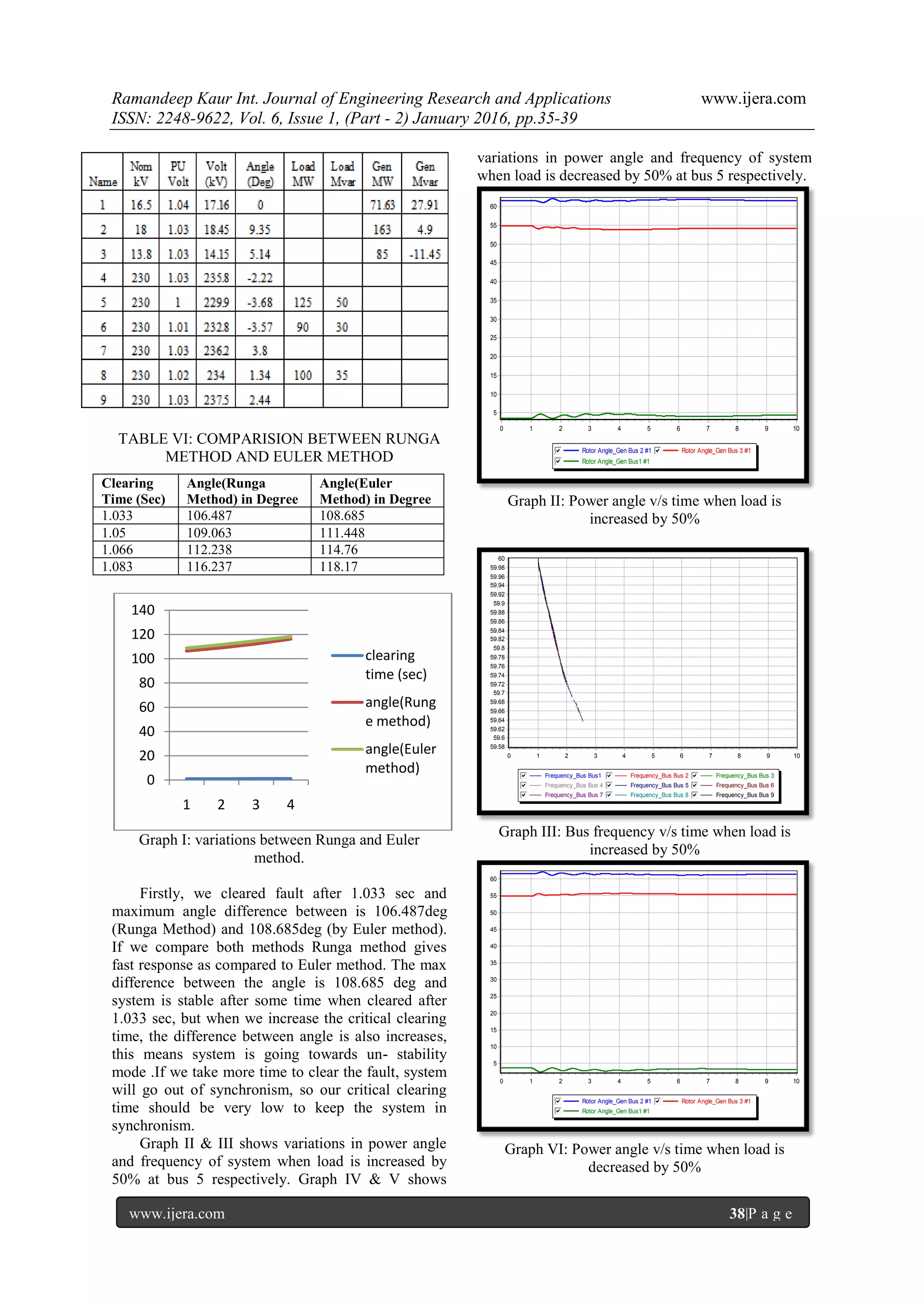
Graph V: Bus frequency v/s time when load is
decreased by 50%
In IEEE 9 BUS MODEL, when sudden load is
increased by 50%, the power angle curves become
unstable and frequency of system suddenly decreases
as shown in graph II & III while when sudden load is
increased by 50%, the power angle curves become
unstable and frequency of system suddenly decreases
as shown in graph IV & V.
IV. CONCLUSION
It is concluded that Power system should have
very low critical clearing time to operate the relays, if
we isolate the faulty section within very short time,
thus system can obtain the stability otherwise it will
go out of synchronism. In this research work, load
flow studies are performed to analyse the transient
stability of system. The behaviour of three phase
balanced fault and impact of load switching is also
investigated. Thus the protection system provided for
the system should have fast response. According to
this analysis, fast fault clearing and load shedding
methodologies can be adopted for system stability.
REFERENCES
[1] R. A. Naghizadeh, S. Jazebi, B. Vahidi,
“Modeling hydro power plants and
tuning hydro governors as an educational
guideline,” International Review on
Modeling and Simulations (I.RE.MO.S.),
Vol. 5, N. 4, August 2012.
[2] Vadim Slenduhhov, Jako Kilter, “Modeling
and analysis of the synchronous generators
excitation systems”, Publication of Doctoral
School of Energy and Geotechnology,
Pärnu, 2013.
[3] Sandeep Kaur, Dr. Raja Singh Khela,
“Power system design & stability analysis,”
international journal of advanced research in
computer science and software engineering,
Volume 4, Issue 1, January 2014.
[4] M.A Salam, M. A. Rashid, Q. M. Rahman
and M. Rizon, “Transient stability analysis
of a three machine nine bus power system
network”, Advance online publication, 13
February 2014.
[5] Swaroop Kumar. Nallagalva, Mukesh
Kumar Kirar, Dr.Ganga Agnihotri,
“Transient Stability analysis of the IEEE 9-
Bus electric power system”, International
Journal of Scientific Engineering and
Technology, Volume No.1, Issue No.3, pp.:
161-166, July 2012.
[6] Ž. Eleschová, M. Smitková and A. Beláň,
“Evaluation of power system transient
stability and definition of the basic
criterion”, Internationals journal of energy,
Issue 1, Vol. 4, 2010.
[7] Tin Win Mon and Myo Myint Aung
“Simulation of synchronous machine in
stability study for power system”,
International Journal of Electrical and
Computer Engineering 3:13, 2008.
[8] Yaman C. Evrenosoglu, Hasan Dag,
“Detailed Model for Power System
Transient Stability Analysis”.
[9] H.T.Hassan, 2Usman Farooq Malik, 3Irfan
Ahmad Khan, 4Talha Khalid, “Stability
Improvement of Power System Using
Thyristors Controlled Series Capacitor
(TCSC)”, International Journal of
Engineering & Computer Science IJECS-
IJENS, Vol: 13 No: 02.
[10] Gundala Srinivasa Rao, Dr.A.Srujana,
“Transient Stability Improvement of Multi-
machine Power System Using Fuzzy
Controlled TCSC” International Journal of
Advancements in Research & Technology”,
ISSN 2278-7763, Volume 1, Issue 2, July-
2012.
[11] Renuka Kamdar, Manoj Kumar and Ganga
Agnihotri, “
Transient Stability Analysis and
Enhancement of Ieee- 9 Bus System”,
Electrical & Computer Engineering: An
International Journal (ECIJ) Volume 3,
Number 2, and June 2014.
Frequency_Bus Bus1gfedcb Frequency_Bus Bus 2gfedcb Frequency_Bus Bus 3gfedcb
Frequency_Bus Bus 4gfedcb Frequency_Bus Bus 5gfedcb Frequency_Bus Bus 6gfedcb
Frequency_Bus Bus 7gfedcb Frequency_Bus Bus 8gfedcb Frequency_Bus Bus 9gfedcb
109876543210
60.38
60.36
60.34
60.32
60.3
60.28
60.26
60.24
60.22
60.2
60.18
60.16
60.14
60.12
60.1
60.08
60.06
60.04
60.02
60