Downloaded 886 times
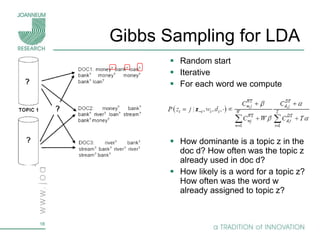
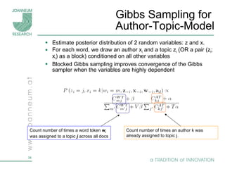


Topic models are probabilistic models for discovering the underlying semantic structure of a document collection based on a hierarchical Bayesian analysis. Latent Dirichlet allocation (LDA) is a commonly used topic model that represents documents as mixtures of topics and topics as distributions over words. LDA uses Gibbs sampling to estimate the posterior distribution over topic assignments given the words in each document.


![[Kim+ ICML2012] Dirichlet Process with Mixed Random Measures : A Nonparametri...](https://cdn.slidesharecdn.com/ss_thumbnails/dp-mrmkimicml2012-120727233419-phpapp01-thumbnail.jpg?width=640&height=640&fit=bounds)