Downloaded 188 times

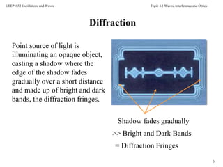
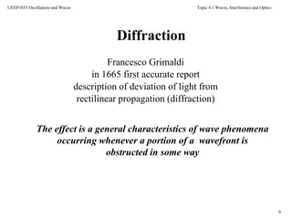
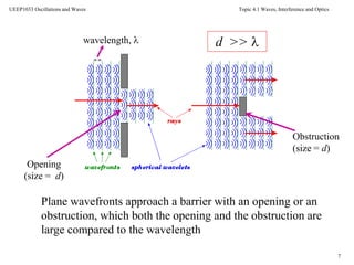

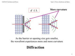

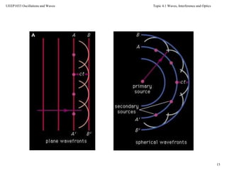
![Topic 4.1 Waves, Interference and Optics
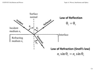
29
UEEP1033 Oscillations and Waves
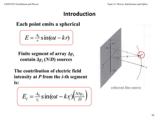
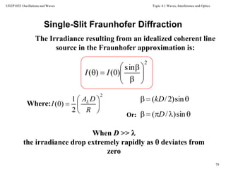
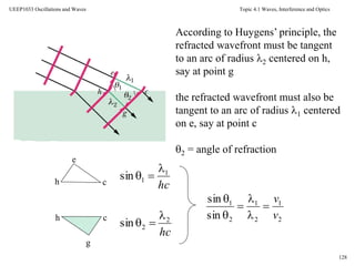
This result can be rewritten as:
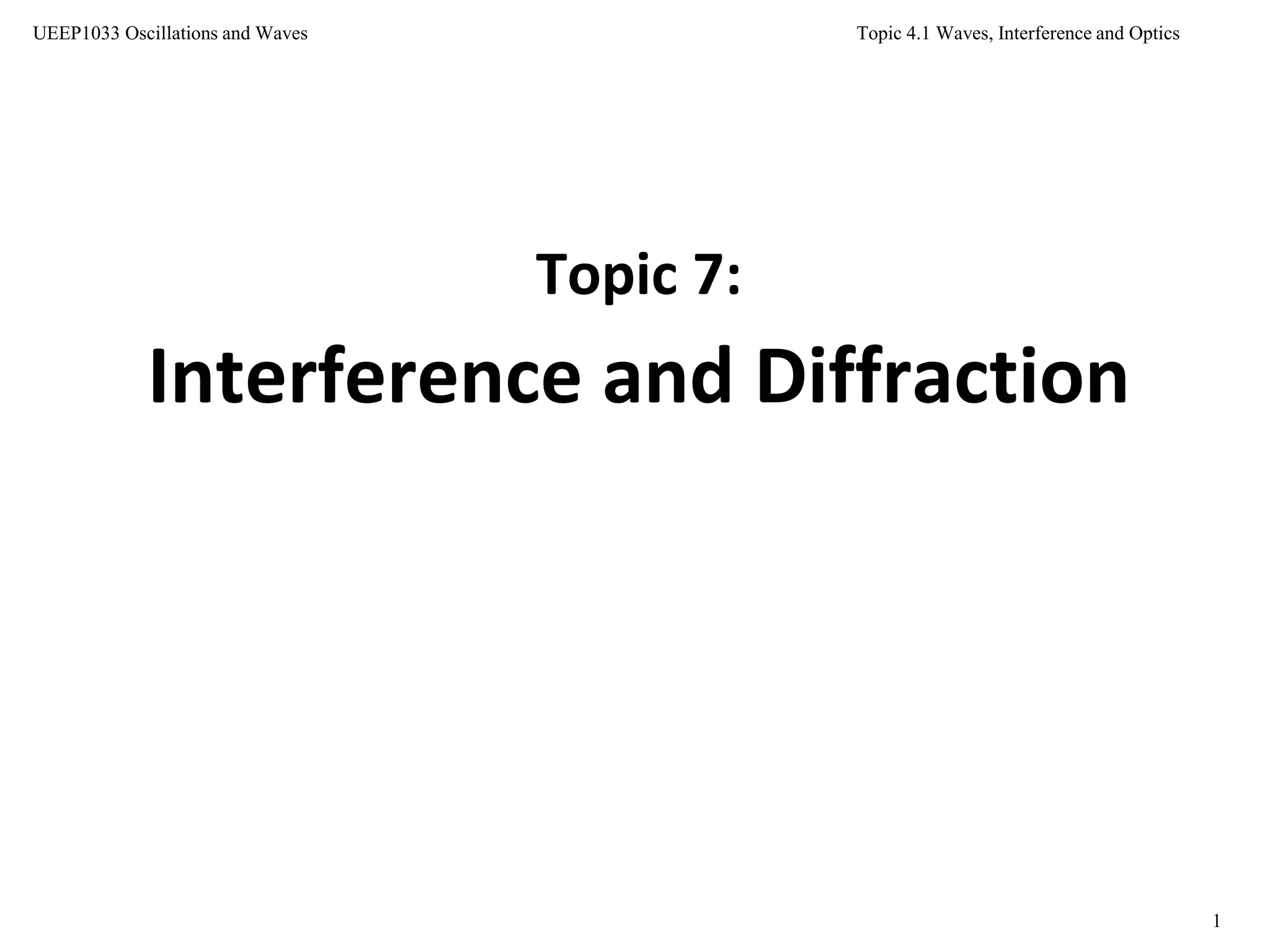
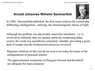
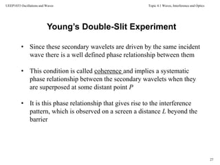
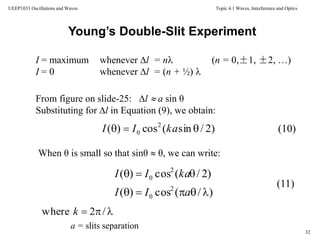
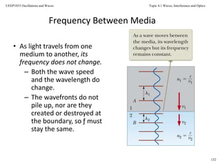
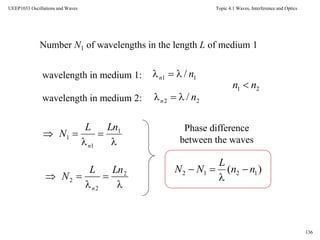
Since L >> a, the lines from S1 and S2 to P can be assumed to be
parallel and also to make the same angle θ with respect to the
horizontal axis
Young’s Double-Slit Experiment
2/)(cos[]2/)(cos2 1212 llkllktAR
The line joining P to the mid-point of the slits makes an angle θ
with respect to the horizontal axis
21 cos/ lLl
cos/212 Lll
(6)
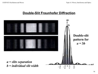
a = slits separation](https://image.slidesharecdn.com/topic7waveinterference-140705124634-phpapp01/85/Topic-7-wave-interference-29-320.jpg)
![Topic 4.1 Waves, Interference and Optics
50
UEEP1033 Oscillations and Waves
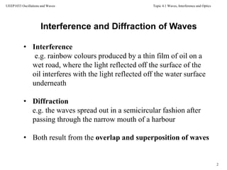
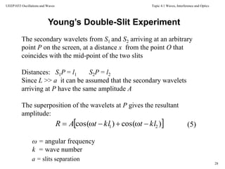
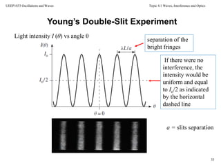
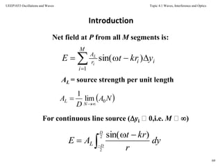
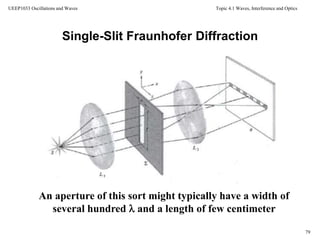
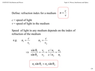
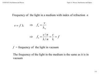
Hence dR is given by:
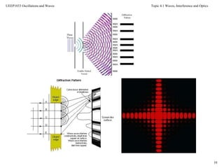
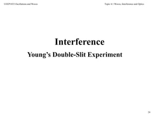
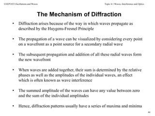
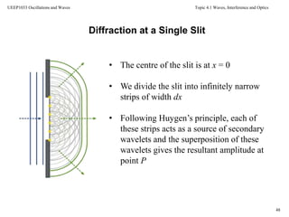
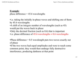
Diffraction at a Single Slit
ω = angular frequency k = wave number α = constant
)]sin(cos[ xlktdxdR
The resultant amplitude at P due to the contributions of the
secondary wavelets from all the strips is
2/
2/
)]sin(cos[
d
d
xlktdxR
)cos(]sin)2/sin[(
sin)2/(
kltkd
kd
d
R
d = slit width](https://image.slidesharecdn.com/topic7waveinterference-140705124634-phpapp01/85/Topic-7-wave-interference-50-320.jpg)
![Topic 4.1 Waves, Interference and Optics
51
UEEP1033 Oscillations and Waves
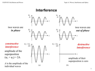
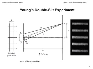
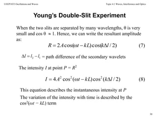
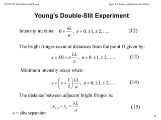
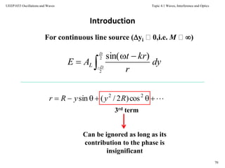
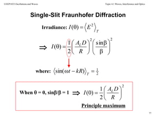
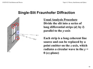
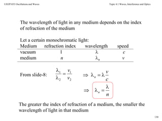
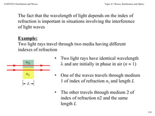
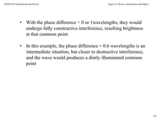
Instantaneous intensity I at P:
2
2
2222
]sin)2/[(
]sin)2/[(sin
)(cos
kd
kd
kltdRI
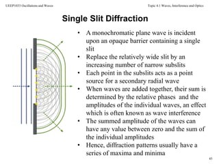
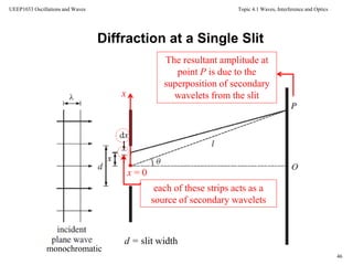
Diffraction at a Single Slit
Since the time average over many cycles of cos2(ωt − kl) = 1/2
the time average of the intensity is given by:
2
2
02
2
0
sin
]sin)2/[(
]sin)2/[(sin
)(
I
kd
kd
II
2/22
0 dI = maximum intensity of the diffraction pattern
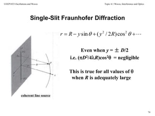
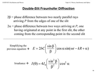
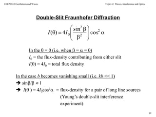
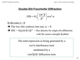
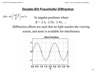
This equation describes how an incident plane wave of wavelength λ
spreads out from a single slit of width d in terms of the angle θ
2/sin kd](https://image.slidesharecdn.com/topic7waveinterference-140705124634-phpapp01/85/Topic-7-wave-interference-51-320.jpg)
![Topic 4.1 Waves, Interference and Optics
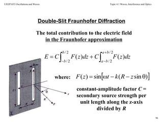
54
UEEP1033 Oscillations and Waves
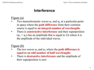
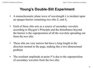
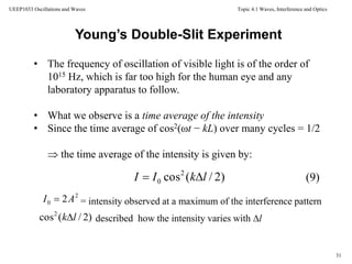
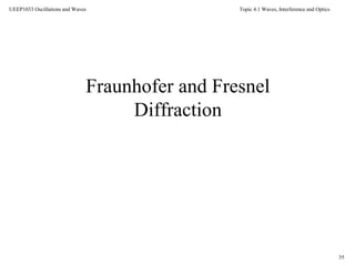
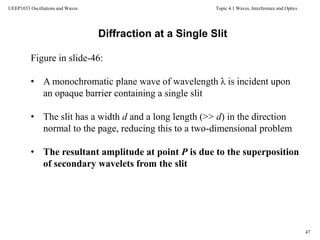
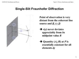
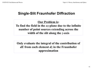
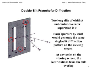
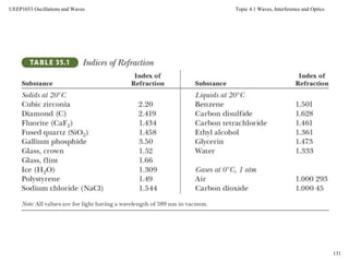
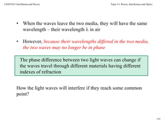
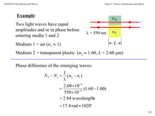
Double slits of finite width
• Consider each of the two slits to be composed of infinitely
narrow strips that act as sources of secondary wavelets
• Then the resultant amplitude R at a point P is the
superposition of the secondary wavelets from both slits
2/2/
2/2/
2/2/
2/2/
)]sin(cos[
)]sin(cos[
da
da
da
da
xlktdx
xlktdxR
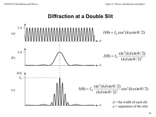
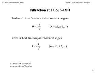
d = the width of each slit
a = separation of the slits](https://image.slidesharecdn.com/topic7waveinterference-140705124634-phpapp01/85/Topic-7-wave-interference-54-320.jpg)
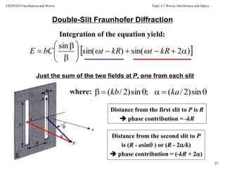
![Topic 4.1 Waves, Interference and Optics
55
UEEP1033 Oscillations and Waves
]sin)2/cos[(
sin)2/(
]sin)2/sin[(
)cos(2
ka
kd
kd
kltdR
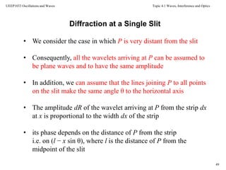
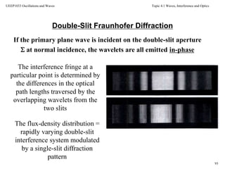
Double slits of finite width
]sin)2/[(cos
]sin)2/[(
]sin)2/[(sin
)( 2
2
2
0
ka
kd
kd
II
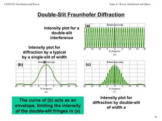
Resultant Intensity:
• This result is the product of two functions.
• The first is the square of a sinc function corresponding to
diffraction at a single slit
• The second is the cosine-squared term of the double-slit
interference pattern](https://image.slidesharecdn.com/topic7waveinterference-140705124634-phpapp01/85/Topic-7-wave-interference-55-320.jpg)
![Topic 4.1 Waves, Interference and Optics
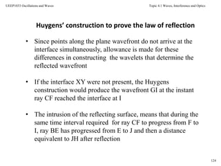
75
UEEP1033 Oscillations and Waves
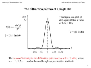
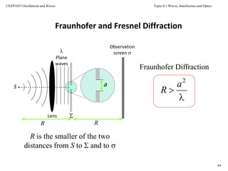
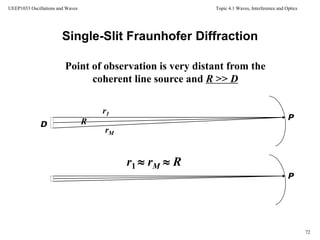
Fraunhofer conditions: The distance r is linear in y
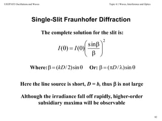
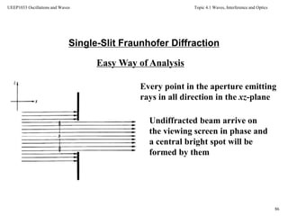
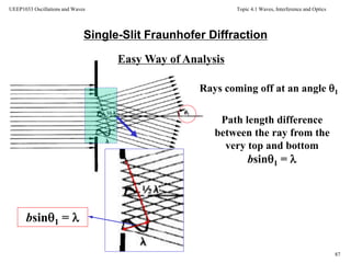
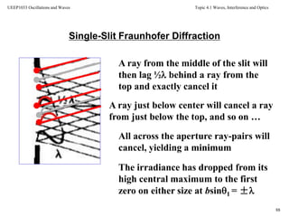
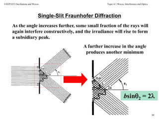
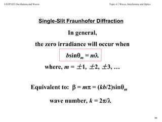
Single-Slit Fraunhofer Diffraction
Therefore the phase can be written as a
function of the aperture variable
sinyRr
dyyRkt
R
A
E
D
D
L
2
2
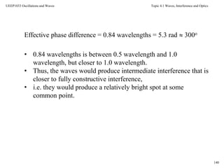
)]sin(sin[
)sin( yRkkr](https://image.slidesharecdn.com/topic7waveinterference-140705124634-phpapp01/85/Topic-7-wave-interference-75-320.jpg)
![Topic 4.1 Waves, Interference and Optics
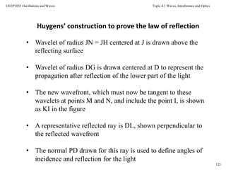
76
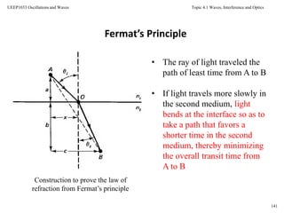
UEEP1033 Oscillations and Waves
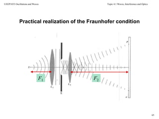
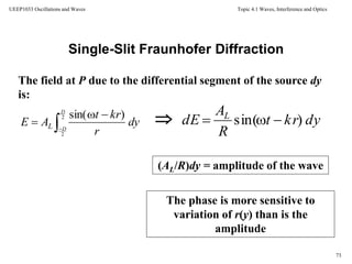
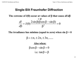
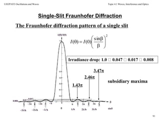
Single-Slit Fraunhofer Diffraction
Simplify:
where:
dyyRkt
R
A
E
D
D
L
2
2
)]sin(sin[
)sin(
sin)2/(
]sin)2/sin[(
kRt
kD
kD
R
DA
E L
)sin(
sin
kRt
R
DA
E L
sin)2/(kD](https://image.slidesharecdn.com/topic7waveinterference-140705124634-phpapp01/85/Topic-7-wave-interference-76-320.jpg)
![Topic 4.1 Waves, Interference and Optics
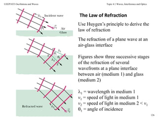
109
UEEP1033 Oscillations and Waves
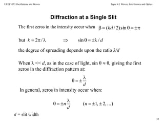
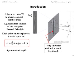
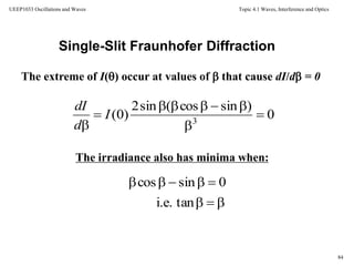
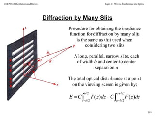
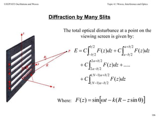
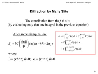
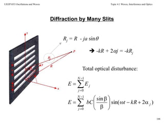
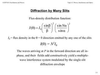
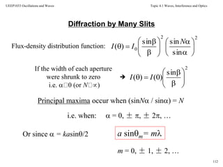
Diffraction by Many Slits
Total optical disturbance written as the
imaginary part of a complex exponential:
Geometric series
1
0
2)(sin
Im
N
j
jikRti
eebCE
][
][
1
1
2
21
0
2
iii
iNiNiN
i
NiN
j
ji
eee
eee
e
e
e
sin
sin)1(
1
0
2 N
ee Ni
N
j
ji](https://image.slidesharecdn.com/topic7waveinterference-140705124634-phpapp01/85/Topic-7-wave-interference-109-320.jpg)
![Topic 4.1 Waves, Interference and Optics
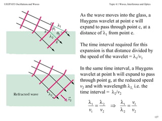
110
UEEP1033 Oscillations and Waves
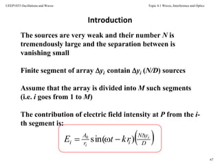
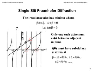
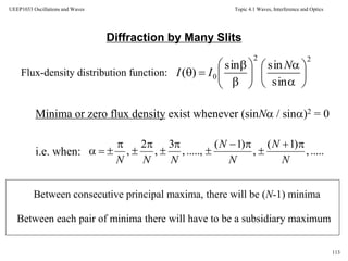
Diffraction by Many Slits
Total optical disturbance written as the
imaginary part of a complex exponential:
1
0
2)(sin
Im
N
j
jikRti
eebCE
])1(sin[
sin
sinsin
NkRt
N
bCE](https://image.slidesharecdn.com/topic7waveinterference-140705124634-phpapp01/85/Topic-7-wave-interference-110-320.jpg)

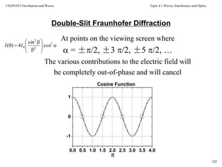
Interference and diffraction are phenomena that occur when two waves overlap and interact. Young's double-slit experiment demonstrated interference by shining light through two slits and observing alternating bright and dark bands in the interference pattern on a screen. The intensity of the bands is determined by the path difference between waves from the two slits, which causes constructive or destructive interference. This experiment provided evidence that light behaves as a wave and established the foundation for optics.


![Polymer [ बहुलक ] Chemistry Notes PDF - Irfanullah Mehar - JJ Sir Chemistry.pdf](https://cdn.slidesharecdn.com/ss_thumbnails/polymerchemistrynotespdf-irfanullahmehar-jjsirchemistry-260210172118-3f9b37f7-thumbnail.jpg?width=640&height=640&fit=bounds)


