A physical derivation of the Boltzmann Transport Equation of kinetic theory, using only basic scattering theory.

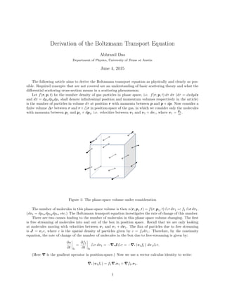
1. Derivation of the Boltzmann Transport Equation
Abhranil Das
Department of Physics, University of Texas at Austin
June 4, 2015
The following article aims to derive the Boltzmann transport equation as physically and clearly as pos-
sible. Required concepts that are not covered are an understanding of basic scattering theory and what the
differential scattering cross-section means in a scattering phenomenon.
Let f(r, p, t) be the number density of gas particles in phase space, i.e. f(r, p, t) dτ dπ (dτ = dxdydz
and dπ = dpxdpydpz shall denote infinitesimal position and momentum volumes respectively in the article)
is the number of particles in volume dτ at position r with momenta between p and p + dp. Now consider a
finite volume ∆τ between r and r + r in position-space of the gas, in which we consider only the molecules
with momenta between p1 and p1 + dp1, i.e. velocities between v1 and v1 + dv1, where v1 = p1
m .
b b+db
g dt
Figure 1: The phase-space volume under consideration
The number of molecules in this phase-space volume is then n(r, p1, t) = f(r, p1, t) τ dπ1 =: f1 r dπ1.
(dπ1 = dp1xdp1ydp1z etc.) The Boltzmann transport equation investigates the rate of change of this number.
There are two causes leading to the number of molecules in this phase space volume changing. The first
is free streaming of molecules into and out of the box in position space. Recall that we are only looking
at molecules moving with velocities between v1 and v1 + dv1. The flux of particles due to free streaming
is J = v1c, where c is the spatial density of particles given by c = f1dπ1. Therefore, by the continuity
equation, the rate of change of the number of molecules in the box due to free-streaming is given by:
∂n
∂t fs
=
∂f1
∂t fs
τ dπ1 = − .J τ = − . (v1f1) dπ1 τ.
(Here is the gradient operator in position-space.) Now we use a vector calculus identity to write:
. (v1f1) = f1 .v1 + f1.v1.
1

2. Now, since over the box we have assumed the velocities v1 of the particles to be constant (velocities don’t
change due to free-streaming, only due to collisions, which will be dealt with later), .v1 = 0 and we have:
∂f1
∂t fs
τ dπ1 = − f1.v1 dπ1 τ ⇒
∂f1
∂t fs
= − f1.v1.
Note that f1.v1 is different from the vector derivative v1. f1.
The second reason for the change of f1 is intermolecular collisions which cause particles to drop into and
out of the momentum volume we are looking at. First we consider particles dropping out of this volume, and
we shall denote the corresponding rate of change by ∂f1
∂t
coll-
. Since the momentum volume we are looking
at is infinitesimal, we assume that particles in that volume undergoing collisions necessarily go out of the
volume (i.e. there are no infinitesimally glancing collisions). First consider the rate of particles scattered
out of the momentum volume by collisions. Consider one of the particles in the box we are looking at, with
momentum p1, suffering a collision p1p2 → p1p2. There are two parameters of such a collision, the impact
parameter and the relative speed before the collision |p1−p2|
m = g(p1, p2). (This is the standard notation in
this context; don’t shoot the messenger.) The average number of collisions undergone in time dt by particle
1 with a particle with momentum p2 and with impact parameter between b and b + db is the number of
particles with momentum p2 in the annular cylindrical volume depicted below (remember that for a general
interparticle potential, ‘collision’ may or may not involve the particles coming in hard sphere contact):
b b+db
g dt
Figure 2: The annular cylinder of collisions
This number is given by 2πb db g dt f2 dπ2 (f2 := f(r, p2, t)). Thus, the rate of such collisions per unit
time is 2πb db g f2 dπ2.
Here is a little catch. Particle 1 does not continue on undeterred through the cylinder after its collisions.
It’s momentum changes after each collision, i.e. both the speed and direction. However, notice that we
have assumed that the distribution of momenta of the particle 2 is entirely statistically independent or
uncorrelated with that of particle 1. This assumption is named ‘molecular chaos’, or Stosszahl-Ansatz as
Boltzmann put it. With this assumption, statistically speaking we can use the above picture of a fixed
cylinder.
To get the total rate of collisions suffered by particle 1, we should integrate over the momentum of the
second particle and the impact parameter of the collision, to get:
ˆ
b
2πb db
ˆ
p2
g(p1, p2) f2 dπ2.
Now, the total number of particles with momentum p1 that this applies to is the number of particles in
the phase-space volume we were looking at, f1 τ dπ1. So we can say that the total rate of change of the
number of particles in the phase-space volume due to collisions removing them from dπ1 is:
∂n
∂t coll-
=
∂f1
∂t coll-
τ dπ1 = −
ˆ
b
2πb db
ˆ
p2
g f1 f2 dπ2 τ dπ1 (1)
⇒
∂f1
∂t coll-
= −
ˆ
b
2πb db
ˆ
p2
g f1 f2 dπ2
2

3. Here the integration over p2 includes automatically the integration over g.
Now, in analogy with 1, the rate of collisions of the form p1p2 → p1p2 introducing particles from outside
into dπ1 is given by:
∂n
∂t coll+
= 2π
ˆ
b
b db
ˆ
p2
g f1 f2 dπ2 r dπ1
But note that for a collision, given p1 and p2 we know p1 and p2 and vice versa uniquely through
bijective functions. So f1 = f(r, p1, t) and f2 = f(r, p2, t) can also be rewritten in terms of p1 and p2 as
their arguments. Assuming such a rewritten function, we can write:
∂n
∂t coll+
=
∂f1
∂t coll+
τ dπ1 = 2π
ˆ
b
b db
ˆ
p2
g f1 f2 dπ2 τ dπ1
In the above, dπ1 and dπ1 represent the same infinitesimal momentum volume of the first colliding
particle under consideration, just from two opposite perspectives. These volumes are therefore same and can
be cancelled. So we get:
∂f1
∂t coll+
= 2π
ˆ
b
b db
ˆ
p2
g f1 f2 dπ2
Now, in ∂f1
∂t
coll-
and ∂f1
∂t
coll+
, instead of integrating over the impact parameter, we can equivalently
integrate over the scattered solid angle once we relate the two using the definition of the differential scattering
cross-section. In the center-of-mass frame, this relation is:
2πb db = σcm(Θ)dΩ,
where Θ and σcm(Θ) are respectively the scattering angle and the differential scattering cross-section in
the center-of-mass frame, and dΩ is the solid angle 2π sin ΘdΘ. (The scattering phenomenon is azimuthally
symmetric.)
Then we can then write:
∂f1
∂t coll-
= −
ˆ
Ω
σcmdΩ
ˆ
p2
g f1 f2 dπ2,
∂f1
∂t coll+
=
ˆ
Ω
σcmdΩ
ˆ
p2
g f1 f2 dπ2
Putting all the terms together then, we get:
∂f1
∂t
=
∂f1
∂t fs
+
∂f1
∂t coll
=
∂f1
∂t fs
+
∂f1
∂t coll+
+
∂f1
∂t coll-
= − f1.v1 +
ˆ
Ω
σcmdΩ
ˆ
p2
g f1 f2 dπ2 −
ˆ
Ω
σcmdΩ
ˆ
p2
g f1 f2 dπ2.
⇒
∂f1
∂t
+ f1.v1 =
ˆ
Ω
σcmdΩ
ˆ
p2
g f1 f2 − f1f2 dπ2.
This is the Boltzmann transport equation.
In the case of elastic collisions, the after-collision momenta p1 and p2 are found uniquely from the
before-collision momenta p1 and p2 using conservation of momentum and energy: p1 + p2 = p1 + p2 and
m1v2
1 +m2v2
2 = m1v 2
1 +m2v 2
2 . So we can express f1 and f2 in terms of their natural arguments p1 and p2 and
write, integrating over all primed momenta and including the conservation constraints using delta-functions:
∂f1
∂t
+ f1.v1 =
ˆ
Ω
σcmdΩ
ˆ
p2
ˆ
p1
ˆ
p2
g f1 f2 − f1f2 δ3
(p1+p2−p1−p2)δ(m1v2
1+m2v2
2−m1v 2
1 +m2v 2
2 )dπ2dπ1dπ2.
3