Downloaded 831 times

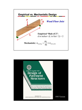
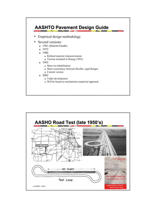
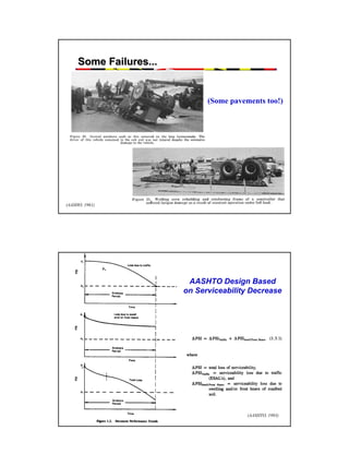
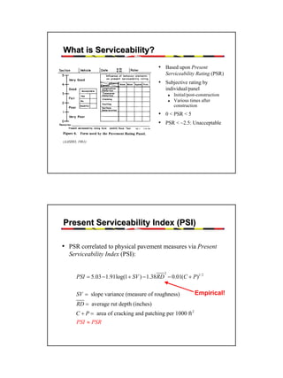
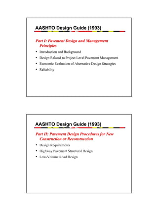
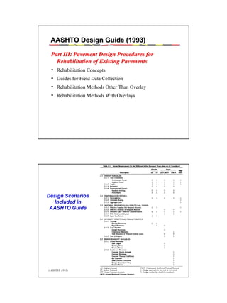

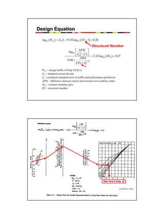
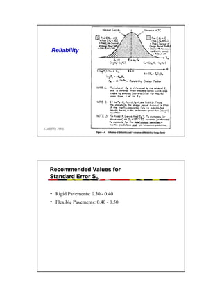
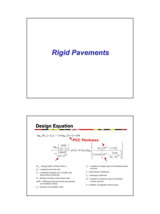
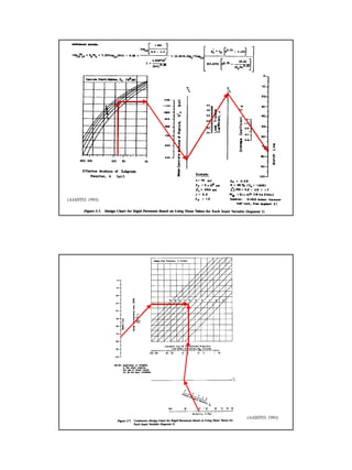
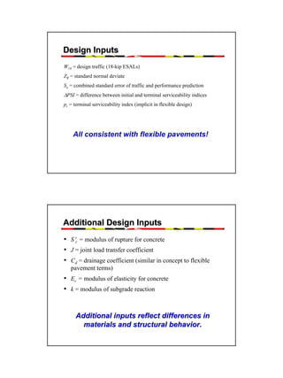

This document provides an overview of pavement design methods and the 1993 AASHTO Guide for pavement design of both flexible and rigid pavements. It summarizes: - The objectives and inputs considered in pavement design - The empirical and mechanistic-empirical approaches used in the AASHTO Guide - The key equations, parameters, and design process for both flexible and rigid pavement structures It describes how the AASHTO Guide is based on predicting the decrease in serviceability over time under traffic loading using reliability concepts. The design process involves calculating the structural number for flexible pavements or slab thickness for rigid pavements based on traffic, materials properties, and reliability factors.


