This document defines and provides examples of supermanifolds by discussing the necessary algebraic concepts. It begins by introducing supermanifolds and noting they are used in physics theories. It then covers the relevant algebra topics needed to define a supermanifold, including graded rings and supercommutative rings. A key example is the ring of polynomials R0|2, which is shown to be a supercommutative ring graded over Z/2. This provides the algebraic framework for defining supermanifolds using category theory and sheaves.

1. SUPERMANIFOLDS
VIA CATEGORIES AND SHEAVES
JAMES HOLBERT
1. INTRODUCTION
In the quest for a theory of everything, physicists use supermani-
folds in their theories of superstrings and supergravity. Mathemati-
cally, what is a supermanifold? Even without being familiar with an
ordinary classical manifold, one can easily understand what a super-
manifold is. We’ll go through what we need from algebra, topology,
category theory, and sheaves, in order to define a supermanifold.
We assume familiarity with basic set theory, e.g., relations, func-
tions, inverse images, unions, intersections, indexed families of sets,
etc. Also, we assume familiarity with collections as generalizations
of sets, as sets are sometimes not large enough. Recall Russell’s para-
dox — is the set R which contains all sets which are not members of
themselves really a set? Maybe not, since R 2 R if and only if R /2 R.
And we assume familiarity with the notion of a commutative dia-
gram, e.g., saying the diagram
A
C
B
D
g
✏✏
j
✏✏
f
//
g
//
commutes means
j f = g g.
1.1. Notation. By f : X ! Y, we denote a map from set X to set Y,
and f : x 7! x3 denotes the function such that f (x) = x3. By Z>0, we
mean the positive integers {1, 2, 3, . . .}.
Date: Spring 2010.

2. JAMES HOLBERT 2
2. ALGEBRA
We first recall some familiar basic algebra definitons and exam-
ples. Then we discuss Z/2-graded rings and supercommutative
rings.
2.1. Definition — Binary Operation. Let S be a set. A binary oper-
ation · is a function S ⇥ S ! S. For example, addition of integers is a
binary operation +: Z ⇥ Z ! Z. As usual, we’ll write a + b instead
of +(a, b).
2.2. Definition — Monoid. A monoid is a pair (M, ·), where M is a
set and · is a binary operation such that
(i) for any a, b, c 2 M,
a · (b · c) = (a · b) · c,
(ii) there exists 1 2 M such that for any a 2 M,
1 · a = a · 1 = a.
We call condition (i) associativity, and we call such a 1 2 M the iden-
tity element. Identities are unique, a simple exercise. We may refer
to just M as a monoid.
2.3. Definition — Group. A group is a monoid (G, ·) with inverses,
i.e., for any g 2 G, there exists g0 2 G such that
g · g0
= g0
· g = 1.
We call such a g0 the inverse of g. Uniqueness is a simple exercise,
and we denote the inverse of g by g 1. Again, we’ll refer to just G as
a group. And we may drop the · notation, i.e., we’ll write ab instead
of a · b.
2.4. Definition — Subgroup. Let G be a group. Then H is a sub-
group of G if and only if
(i) H 6= ∆,
(ii) if a, b 2 H, then ab 2 H,
(iii) if a 2 H, then a 1 2 H.
2.5. Example. The set of all integers Z with addition is a group, and
the set of all even integers 2Z is a subgroup of Z.

3. JAMES HOLBERT 3
2.6. Definition — Abelian Group. An abelian group is a group G
such that for any a, b 2 G,
ab = ba.
We call this property commutativity. Typically, we denote the iden-
tity in an abelian group by 0 and the inverse of a by a.
2.7. Examples. The set of all real n ⇥ n matrices with matrix mul-
tiplication is a monoid. Multiplying two real n ⇥ n matrices yields
an n ⇥ n real matrix. Matrix multiplication is associative. And the
identity matrix is just the matrix with 1s on the diagonal and zeros
everywhere else.
The set of all nonsingular, i.e., invertible, real n ⇥ n matrices with
matrix multiplication is a group but not an abelian group. Matrix
multiplication is certainly not commutative in general.
But the set of all real n ⇥ n matrices with matrix addition is an
abelian group.
2.8. Definition — Ring. A ring is a triple (R, +, ·) such that
(i) (R, +) is an abelian group,
(ii) (R, ·) is a monoid,
(iii) for any a, b, c 2 R,
a(b + c) = ab + ac, (a + b)c = ac + bc.
We call condition (iii) distributivity. Recall we drop the · notation,
writing ab instead of a · b. We call + addition and · multiplication.
We denote the additive identity by 0, which we call the zero, and we
denote the multiplicative identity by 1, which we call the unit.
Ring terminology is not universally accepted. In particular, some
definitions do not require a multiplicative identity. But, here, when
we say ring, we do assume a unit. And some call 1 the unity element
and any element with a multiplicative inverse a unit. Sometimes,
associativity of multiplication is not even assumed.
2.9. Theorem. Let R be a ring. Then for any r 2 R, 0r = 0.
Proof. Let r 2 R. Since 0 = r r, by distributivity, 0r = (r r)r =
r2 r2 = 0. ⇤
2.10. Example — Ring of Functions RS. Let S be a set. Then the set
of all functions
RS
= {f | f : S ! R}
with pointwise addition and multiplication, i.e., for any p, q 2 S,
f + g: p 7! f (p) + g(p), f g: p 7! f (p)g(p)

4. JAMES HOLBERT 4
is a ring. The zero and unit functions are the constant functions
0: p 7! 0, 1: p 7! 1.
2.11. Example — Z/2. Let Z/2 = {0, 1} with 0 as the zero and 1 as
the unit, along with
1 + 1 = 0.
Then Z/2 is a ring.
2.12. Definition — Ideal. Let R be a ring. Then I is an ideal of R if
and only if
(i) (I, +) is a subgroup of (R, +),
(ii) for any r 2 R and any a 2 I, ra 2 I,
(iii) for any r 2 R and any a 2 I, ar 2 I.
We could write conditions (ii) and (iii) as
RI ✓ I ◆ IR.
We say an ideal I is proper if and only if I 6= R.
2.13. Example. Let 2Z = {2n 2 Z | n 2 Z}. Then 2Z is an ideal of
Z. Indeed, (2Z, +) is a subgroup of (Z, +), and for any m 2 Z and
any 2n 2 2Z,
m · 2n = 2n · m = 2(mn) 2 2Z,
i.e., 2Z ✓ Z ◆ 2Z.
2.14. Definition — Maximal Ideal. Suppose M is an ideal of ring R.
Then M is a maximal ideal if and only if M 6= R and the only ideal
containing M is either M or R.
2.15. Example. Consider the ring Z Let p 2 Z be prime and
pZ = {pa 2 Z | a 2 Z}.
Then pZ is a maximal ideal. Let a, b 2 pZ with a = pm and b = pn.
Then a b = p(m n) 2 Z, so (pZ, +) is a subgroup of (Z, +).
And for any k 2 Z, ka = kpm = p(km) = ak 2 pZ, so
Z(pZ) ✓ pZ ◆ (pZ)Z.
Thus pZ is an ideal of Z. Note pZ 6= Z since 1 /2 pZ. To see pZ
is maximal, we recall each ideal in Z is principal, i.e., generated by
one element, because each subgroup of (Z, +) is generated by one
element. Thus, because p is prime and gcd(p, a) is either 1 or p, no
other proper ideal contains pZ.

5. JAMES HOLBERT 5
2.16. Definition — Ring Homomorphism. A map j: R ! S is a
ring homomorphism if and only if
(i) R and S are rings,
(ii) if a, b 2 R, then j(a + b) = j(a) + j(b),
(iii) if a, b 2 R, then j(ab) = j(a)j(b),
(iv) j(1) = 1.
2.17. Definition — Z/2-graded Ring. Let R be a ring with two ad-
ditive subgroups R0 and R1 such that for any r 2 R, there exists
a 2 R0 and b 2 R1 such that r = a + b. For i, j 2 Z/2, define
RiRj = {ab 2 R | a 2 Ri, b 2 Rj}.
We call R a Z/2-graded ring if and only if
RiRj ✓ Ri+j,
for any i, j 2 Z/2.
We call the elements of R0 even, the elements of R1 odd, and the
elements of R0 [ R1 pure (or homogeneous). And we may write
R = R0 R1.
2.18. Example — C as a Z/2-graded Ring. Recall the complex num-
bers
C = {a + bi | a, b 2 R, i2
= 1}
with addition and multiplication for any x + yi, u + vi 2 C given by
(x + yi) + (u + vi) = (x + u) + (y + v)i,
(x + yi)(u + vi) = (xu yv) + (xv + yu)i.
Set
C0 = {a + bi | b = 0}, C1 = {a + bi | a = 0}.
That is, C0 is the real axis and C1 the imaginary axis. Then for i, j 2
Z/2, we get CiCj ✓ Ci+j. Also note for any a + bi 2 C, a 2 C0 and
b 2 C1. Thus C = C0 C1 is a Z/2-graded ring.
2.19. Definition — Parity function #. Let R = R0 R1 be a Z/2-
graded ring. Then the parity function #: R0 [ R1 ! Z/2 is defined
by r 7! i if and only if r 2 Ri.

6. JAMES HOLBERT 6
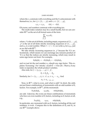
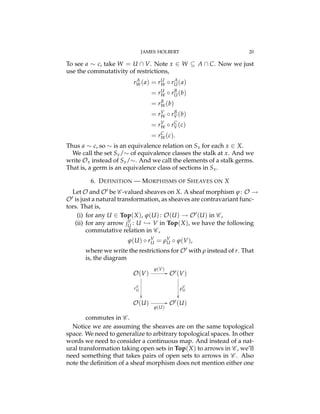
2.20. Theorem. Let R be a Z/2-graded ring. If a and b are pure
elements of R, then #(ab) = #(a) + #(b).
Proof. This is just an interpretation of RiRj ✓ Ri+j. The parity of a
product is the sum of the parities of the factors. To be sure, let a 2 Ri
and b 2 Rj, so ab 2 RiRj ✓ Ri+j. Thus
#(ab) = i + j = #(a) + #(b).
⇤
2.21. Definition — Supercommutative Ring. Let R be a Z/2-graded
ring. Then R is a supercommutative ring if and only if for any pure
a, b 2 R,
ab = ( 1)#(a)#(b)
ba.
2.22. Example — R0|2. Consider the ring of polynomials R0|2 ⌘
R[q1, q2], where
qiqj = qjqi
for i, j 2 {1, 2} and for any a 2 R,
aqi = qia.
Note q2
i = 0 because
q2
i =
1
2
(q2
i + q2
i ) =
1
2
(q2
i q2
i ) =
1
2
· 0 = 0.
Thus, any product of q1 and q2 with three or more factors vanishes,
e.g.,
q1q2q1 = q1q1q2 = q2
1q2 = 0 · q2 = 0.
Set
R0 = {a0 + a12q1q2 | a1, a12 2 R},
R1 = {a1q1 + a2q2 | a1, a2 2 R}.
For any
p = p0 + p1q1 + p2q2 + p12q1q2 2 R,
with pi 2 R for i 2 {0, 1, 2, 12}, we have
p = (p0 + p12q1q2) + (p1q1 + p2q2),
where
p0 + p12q1q2 2 R0, p1q1 + p2q2 2 R1.
That is, for any p 2 R, there exists r 2 R0 and s 2 R1 such that
p = r + s.
Now, to see RiRj ✓ Ri+j, let
p = p0 + p12q1q2, q = q0 + q12q1q2

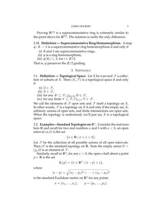
7. JAMES HOLBERT 7
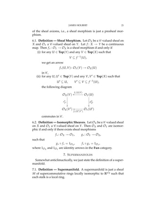
be arbitrary elements of R0, with p0, p12, q0, q12 2 R, and
r = r1q1 + r2q2, s = s1q1 + s2q2,
arbitrary elements of R1, with r1, r2, s1, s2 2 R. Then
pq = (p0 + p12q1q2)(q0 + q12q1q2)
= p0q0 + (p0q12 + p12q0)q1q2,
so R0R0 ✓ R0. And since
pr = (p0 + p12q1q2)(r1q1 + r2q2) = (p0r1)q1 + (p0r2)q2
is odd, we have R0R1 ✓ R1. Similarly, R1R0 ✓ R1. Finally,
rs = (r1q + r2q2)(s1q1 + s2q2) = (r1s2 r2s1)q1q2
is even, so R1R1 ✓ R0. Thus R0|2 is a Z/2-graded ring.
To show supercommutativity, we’ll show evens commute with
everything and odds anticommute with themselves. That is, we
have four cases to cover, and we’ll cover three cases — even·even,
even·odd, and odd·even — with one proof. Then we’ll do the odd·odd
case. So let
t = t0 + t1q1 + t2q2 + t12q1q2
be an arbitrary element in R0|2, i.e., ti 2 R for i 2 {0, 1, 2, 12}. Now
pt = p0t0 + (p0t1)q1 + (p0t2)q2 + (p0t12 + p12t0)q1q2
= t0p0 + (t1p0)q1 + (t2p0)q2 + (t12p0 + t0p12)q1q2
= tp,
so evens commute with everything. That is, if a is even and b is either
even or odd, then
ab = ( 1)#(a)#(b)
ba,
because #(a) = 0, #(a)#(b) = 0, and ( 1)#(a)#(b) = 1. Finally, we
verify odds anticommute. Just note
rs = (r1s2 r2s1)q1q2 = (s1r2 s2r1)q1q2 = sr = ( 1)#(r)#(s)
sr.
We’re done; R0|2 is a supercommutative ring.
2.23. Example — Rp|q. We just generalize R0|2. We now have some
indeterminates xi which commute, along with the familiar anticom-
muting qj. Let p, q be nonnegative integers. Rp|q is just the ring of
polynomials
R[x1, . . . , xp; q1, . . . , qq],

8. JAMES HOLBERT 8
where the xi commute with everything and the qj anticommute with
themselves, i.e., for i, j 2 {1, . . . , p} and r, s 2 {1, . . . , q},
xixj = xjxi, qrqs = qsqr.
Of course, real numbers commute with everything too.
The multi-index notation may be a small hurdle, but we can con-
sider Rp|q as the set of all formal sums of the form
Â
I2I
J2J
aIJxIqJ,
where I is the set of all finite, including empty, sequences of {1, . . . , p},
J is the set of all finite strictly increasing sequences of {1, . . . , q},
and aIJ is a real number. When I = J = ∆, we write a0 for a∆∆, just
as we did with R0|2.
We take strictly increasing sequences in J because the ‘qi’s an-
ticommute, which means we can rearrange any nonzero product of
‘qi’s so that the indices are strictly increasing, which may result in
some sign factor out front. For example,
q3q4q2q1 = q1q3q4q2 = q1q2q3q4,
and we just let the real number aIJ absorb any sign factor. This ex-
plains ‘increasing’. For ‘strictly’, recall q2
i = 0 for all i. That is, if any
index is repeated, the whole product vanishes.
Also note, for J = (j1, j2, . . . , jk) 2 J ,
qJ ⌘ qj1
qj2
· · · qjk
.
Similarly, for I = (i1, . . . , in) 2 I , xI ⌘ xi1
· · · xin
. And
aIJ ⌘ ai1···inj1...jk
.
Now, in Rp|q, what is even, and what is odd? In short, the odds
are just linear combinations of monomials with an odd number of qi
factors. For example, in R9|9, all the monomials
5x2q1q6q8, x6x9q2, pq3q6q7q8q9,
are odd. Likewise, the evens are linear combinations of monomials
who have an even number of qi factors, including no qi factors at all,
e.g.,
5x2q1q4, x6x9, pq2q3q5q8.
In particular, any monomial with no qi factors, including all the real
numbers, is even. Compare this to the definitions of R0 and R1 in
our R0|2 example above.

9. JAMES HOLBERT 9
Proving Rp|q is a supercommutative ring is extremely similar to
the proof above for R0|2. The notation is really the only difference.
2.24. Definition — Supercommutative Ring Homomorphism. A map
j: R ! S is a supercommutative ring homomorphism if and only if
(i) R and S are supercommutative rings,
(ii) j is a ring homomorphism,
(iii) j(Ri) ✓ Si for i 2 Z/2.
That is, j preserves the Z/2 grading.
3. TOPOLOGY
3.1. Definition — Topological Space. Let X be a set and T a collec-
tion of subsets of X. Then (X, T ) is a topological space if and only
if
(i) ∆ 2 T ,
(ii) X 2 T ,
(iii) for any U ✓ T ,
S
U2U U 2 T ,
(iv) for any finite V ✓ T ,
T
V2V V 2 T .
We call the elements of T open sets and T itself a topology on X.
In other words, T is a topology on X if and only if the empty set, X,
arbitrary unions of open sets, and finite intersections are open sets.
When the topology is understood, we’ll just say X is a topological
space.
3.2. Examples—Standard Topologies on Rn. Consider the real num-
bers R and recall for two real numbers a and b with a < b, an open
interval (a, b) is the set
{x 2 R | a < x < b}.
Let T be the collection of all possible unions of all open intervals.
Then sT is the standard topology on R. Note the empty union ∆ =S
∆ U is an element of T .
Similarly, recall in Rn, for any # > 0, the open #-ball about a point
p 2 R is the set
B#(p) = {x 2 Rn
| |x p| < #},
where
|x p| =
q
(x1 p1)2 + · · · + (xn pn)2
is the standard Euclidean metric on Rn for any points
x = (x1, . . . , xn), p = (p1, . . . , pn).

10. JAMES HOLBERT 10
3.3. Definition — Continuous Function. Let X and Y be topological
spaces. Then f : X ! Y is continuous if and only if for any open set
V ✓ Y, the inverse image f 1(V) ✓ X is an open set.
3.4. Definition — Open Cover. Let X be a topological space and
U ✓ X. Then a indexed family {Ua | a 2 A } of sets is an open cover
of U if and only if
(i) each Ua is an open set,
(ii)
[
a2A
Ua = U.
3.5. Definition — Hausdorff. Let X be a topological space. Then X
is Hausdorff if and only if for any two distinct points p, q 2 X, there
are open sets U and V such that
(i) U 6= ∆,
(ii) V 6= ∆,
(iii) p 2 U,
(iv) q 2 V,
(v) U V = ∆.
3.6. Example. The standard topologies on Rn for n 0 are Haus-
dorff.
3.7. Definition — Second Countable. Let X be a topological space.
Then X is second countable if there is a countable basis for the topol-
ogy on X.
4. CATEGORIES
Here, we are using categories mainly just for the language to talk
about sheaves and for a taste of how the subject generalizes math-
ematics into an abstract setting where we focus on arrows between
objects, e.g., group homomorphisms But category theory is a subject
in its own right, with active research in generalized categories called
n-categories.
4.1. Definition — Category. A category C consists of
(i) a collection Ob C ,
(ii) for any A, B 2 Ob C , a set Mor(A, B),
(iii) for any A, B, C 2 Ob C , a function
ABC : Mor(A, B) ⇥ Mor(B, C) ! Mor(A, C).

11. JAMES HOLBERT 11
We call the elements of Ob C objects, and we may write just A 2 C
to indicate A is an object. We call the elements of Mor(A, B) arrows
(or morphisms) from A to B, and we call Mor(A, B) a Mor-set. Some
authors may say Hom-set instead of Mor-set and write Hom(A, B)
instead of Mor(A, B). And as the notation suggests, we call the func-
tions ABC compositions of arrows.
Let’s develop some notation before we see the rest of the defining
conditions for a category. If A, B 2 C are objects and f 2 Mor(A, B)
an arrow from A to B, we may write either
f : A ! B or A
f
! B
to indicate such. And to be clear where these things live, we may say
something like “consider
A
f
! B
g
! C
in C .” And if we are working with more than one category and need
to indicate which category a Mor-set belongs to, we may write
MorD (A, B)
to show we are talking about a Mor-set in category D.
For compositions, we’ll use familiar notation from ordinary func-
tion compositions. But note, in general, arrows are not necessarily
functions or even relations; they are just elements of a set. That is,
given objects and arrows
A
f
! B
g
! C,
instead of writing
ABC(f, g)
for the image of (f, g) 2 Mor(A, B) ⇥ Mor(B, C) under the composi-
tion map ABC, we’ll write
g f,
just as we do with ordinary compositions of functions.
Now, in order for C to be a category, the following conditions must
also hold.
(iv) For any objects and arrows
A
f
! B
g
! C
h
! D,
h (g f ) = (h g) f.

12. JAMES HOLBERT 12
(v) For each A 2 C , there exists 1A 2 Mor(A, A) such that for
any
Z
f
! A
g
! B,
we have
1A f = f, g 1A = g.
In other words, categories just abstract the ideas of sets and func-
tions. We call 1A the identity arrow for A. Compare this with the
definition of a monoid.
4.2. Foundational Warning. You should be concerned about the set-
theoretic foundations of the above definition. We won’t discuss such
issues. MacLane and Awodey address these issues well.
4.3. Examples. To describe a category we just describe its objects, ar-
rows, and how we compose arrows. If the arrows are ordinary func-
tions, we’ll assume compositions of arrows are just ordinary function
compositions. Thus, many examples are nearby.
(i) Set, whose objects are sets and arrows are functions,
(ii) Gp, whose objects are groups and arrows are group homo-
morphisms,
(iii) Rg, whose objects are rings and arrows are ring homomor-
phisms,
(iv) Top, whose objects are topological spaces and arrows are con-
tinuous maps.
4.4. Example — The Dual Category C . Sometimes this category
is denoted C op because the arrows go the opposite direction. Duality
is a theme in category theory, as it is in mathematics in general.
To be precise, let C be a category. We construct the dual category
C by taking the objects of C as the objects of C . And for any
objects A and B,
MorC (A, B) = MorC (B, A).
That is, the arrows A ! B in C are the arrows B ! A in C . Com-
positions get reversed too. For example, the composition g f in
C
A B
C
f
//
g
✏✏
g f
????????????

13. JAMES HOLBERT 13
is just the composition f g
A B
C
f
oo
g
OO
f g
__????????????
in C . Associativity and identities come directly from C . So C is a
category.
4.5. Example — The Category of Open Sets and Inclusions. We’ll
mainly deal with two categories in particular. The first is Top(X),
where X is some fixed topological space. The objects in Top(X) are
the open sets of X. The arrows are inclusion maps. That is, for U, V 2
Top(X), i.e., for any two open sets U and V,
Mor(U, V) =
(
{jV
U} if U ✓ V,
∆ if U 6✓ V,
where jV
U : U ,! V is the inclusion map defined by
U 3 u 7! u 2 V.
Since the inclusion maps are just ordinary functions, Top(X) satisfies
conditions (iv) and (v) in the definition of a category and is thus a
category.
4.6. Example — The Category of Supercommutative Rings. The
category of supercommutative rings SCRg has all supercommuta-
tive rings as objects. And supercommutative ring homomorphisms
are the arrows. Recall a supercommutative ring homomorphism is
just a ring homomorphim preserving the Z/2-grading.
4.7. Functors. Let C and D be categories. A functor F: C ! D is an
assignment such that
(i) for any A 2 Ob C ,
F(A) 2 Ob D,
(ii) for any f : A ! B in C ,
F(f ): F(A) ! F(B),
(iii) for any f : A ! B and any g: B ! C in C ,
F(g f ) = F(g) F(f ),

14. JAMES HOLBERT 14
(iv) for any A 2 C ,
F(1A) = 1F(A).
In other words, a functor maps objects to objects and arrows to ar-
rows, preserving compositions and identity arrows. Such a functor
is called covariant, referring to the preservation of the direction of
the arrows.
A functor which reverses the direction of the arrows is called con-
travariant, which is what we’ll be chiefly concerned with here. To be
sure, the defining conditions of a contravariant functor F: C ! D
are (i) and (iv) above, but we have to replace conditions (ii) and (iii)
with
(ii’) for any f : A ! B in C ,
F(f ): F(B) ! F(A),
(iii’) for any f : A ! B and any g: B ! C in C ,
F(g f ) = F(f ) F(g).
If we say just ‘functor’, we mean covariant, and if we mean con-
travariant, we’ll explicitly say so. Note we could just say F: C ! D
is a contravariant functor if and only if F: C ! D is a functor.
4.8. Example — Forgetful Functor. The forgetful functor on Gp
F: Gp ! Set
takes a group G to the set G and any group homomorphism
j: G ! H
to the function j: G ! H. That is, F forgets the group structure and
just leaves us with the set structure.
4.9. Example — Homology and Cohomology. (We assume famil-
iarity with Algebraic Topology.) The singular homology of a topo-
logical space is a covariant functor, while singular cohomology is a
contravariant functor.
4.10. Definition — Faithful Functor. A functor F: C ! D is faith-
ful if and only if for any
f, g: A ! B
in C such that
F(f ) = F(g): F(A) ! F(B),
in D, we have f = g. Compare this to the definition of an injective
ordinary function. Examples are the forgetful functors on Gp, Rg,
Top, etc.

15. JAMES HOLBERT 15
4.11. Definition — Concrete Category. A concrete category is cat-
egory for which there is a faithful functor F: C ! Set. In other
words, we can think of the objects in C as sets with some structure
possibly and the arrows as ordinary functions.
4.12. Definition — Natural Transformation. Let F, G: C ! D be
functors. Then t : F ! G is a natural transformation if and only if
(i) for any A 2 C ,
t(A): F(A) ! G(A),
(ii) for any f : A ! B in C , the diagram
F(A)
F(B)
G(A)
G(B)
F(f )
✏✏
G(f )
✏✏
t(A)
//
t(B)
//
commutes, i.e.,
G(f ) t(A) = t(B) F(f ).
In other words, a natural transformation maps objects to arrows and
arrows to commutative squares. In a sense, a natural transformation
takes things up a dimension, considering objects as 0-dimensional,
arrows as 1-dimensional, and squares as 2-dimensional, whereas a
functor keeps everything in the same dimension.
4.13. Example — Category of Functors. With natural transforma-
tions, we can construct a category Fun whose objects are functors
and whose arrows are natural transformations. Compositions of nat-
ural transformations, however, are subtle.
Let F, G, H : C ! D be functors. Suppose t : F ! G and n: G !
H are natural transformations. The composition n t : F ! H is
defined by assigning for any A 2 C , the arrow
n t(A) ⌘ n(A) t(A)
in D. Recall t(A): F(A) ! G(A) and n(A): G(A) ! H(A) are
arrows in D for which the composition is defined. We need to verify

16. JAMES HOLBERT 16
the following diagram for any f : A ! B in C
F(A)
F(B)
H(A)
H(B)
F(f )
✏✏
H(f )
✏✏
n t(A)
//
n t(B)
//
commutes. But this follows directly since t and n are natural trans-
formations, which means for any f : A ! B, the diagram
F(A) G(A) H(A)
F(B) G(B) H(B)
F(f )
✏✏
G(f )
✏✏
H(f )
✏✏
t(A)
//
n(A)
//
t(B)
//
n(B)
//
commutes, i.e.,
H(f ) n(A) t(A) = n(B) t(B) F(f ).
Thus, since n(A) t(A) = n t(A) and n(B) t(B) = n t(B), we
get
H(f ) (n t(A)) = (n t(B)) F(f ),
which is precisely what we need for n t to be a natural transforma-
tion from F to H.
Compare this to ordinary function composition, where we have
g f (x) = g(f (x)) for f : X ! Y and g: Y ! Z.
Identity arrows in Fun are slightly subtle too. Let F: C ! D be
a functor, i.e., an object in Fun. Then 1F : F ! F is given for any
A 2 Ob C by
1F(A) = 1F(A),
that is, 1F(A) is the identity arrow in MorD (F(A), F(A)).
4.14. Sheaves and Fun. Sheaves, which we define below, are certain
functors. And we’ll want a notion of isomorphic sheaves, so we’ll
need to know how to compose morphisms of sheaves. This is why
we’re talking about natural transformations and their compositions.

17. JAMES HOLBERT 17
5. SHEAVES
5.1. Definition — Presheaf. Suppose C is a concrete category. A
C -valued presheaf O on topological space X is just a contravariant
functor O : Top(X) ! C . For any open set U ✓ X, we call elements
of O(U) sections. For an inclusion jV
U : U ,! V in Top(X), we write
rV
U for the image O(jV
U) and call rV
U a restriction. Note that since C is
concrete, the restrictions are really ordinary functions.
5.2. Definition — Sheaf. A C -valued sheaf O on topological space
X is just a presheaf O : Top(X) ! C such that for any open set
U ✓ X and any open cover
{Ua ✓ X | a 2 A }
of U,
(i) if s, s0 2 O(U) such that for any a 2 A ,
rU
Ua
(s) = rU
Ua
(s0
),
then s = s0,
(ii) if {sa 2 O(Ua) | a 2 A } is a family of sections such that for
any a, b 2 A ,
rUa
UaUb
(sa) = r
Ub
UaUb
(sb),
then there exists s 2 O(U) such that for all a 2 A ,
rU
Ua
(s) = sa.
We call (i) the separation condition and (ii) the gluing condition. To-
gether, (i) and (ii) are usually called the sheaf axioms. In other words,
for the separation condition, if two sections agree on all the restric-
tions, they are the same section. And for the gluing condition, if
restrictions agree on overlaps for a family of sections {sa 2 O(Ua)},
then all the sections come from a section in U. See the diagrams on
the following page.
5.3. Example — C•. Recall if U ✓ Rn is an open set, a smooth func-
tion U ! R is smooth if and only if all its partial derivatives exist
and are continuous. We show
C•
: Top(Rn
) ! Rg
is a sheaf of rings. Recall Example 2.10. So for each open set U ✓ Rn
C•
(U) = {f : U ! R | f is smooth}

18. JAMES HOLBERT 18
is a ring of smooth functions with pointwise addition and multipli-
cation. Note, in particular, if f, g 2 C•(U), then f + g, f g 2 C•(U).
So this is how the sheaf C• assigns objects to objects Top(Rn) ! Rg.
Now, for any open sets U, V ✓ Rn, the sheaf C• takes the inclusion
arrow jV
U : U ,! V to the restriction
rV
U : C•
(V) ! C•
(U), f 7! f |U,
where f |U : U ! R is the ordinary restriction of f : V ! R given
by U 3 u 7! f (u) 2 R, which is well-defined since U ✓ V and f is
defined for all v 2 V. Since we’re working with ordinary functions
here, we have C• as a presheaf.
Next, we show the sheaf axioms for C•. Actually, the hypotheses
of the separation and gluing conditions are fairly strong, or at least
give us a lot to work with. Suppose U ✓ Rn is an open set and
{Ua | a 2 A }
is an open covering of U. For the separation condition, let f, g 2
C•(U) such that for each a 2 A ,
rU
Ua
(f ) = rU
Ua
(g).
From now on, we’ll write, e.g., f |Ua instead of rU
Ua
(f ). That is, we’re
assuming for each a 2 A ,
f |Ua = g|Ua .
Now, we want to show f = g. Since f, g are just smooth functions
U ! R, suppose x 2 U. Choose w 2 A such that x 2 Uw. Such an
w exists since {Ua|a 2 A } is an open cover. Now
f (x) = f |Uw (x) = g|Uw (x) = g(x).
Hence f = g because x 2 U was arbitrary.
Finally, for the gluing condition, keep U and {Ua | a 2 A } as above.
Suppose
{fa 2 C•
(Ua) | a 2 A }
is a family of smooth functions such that for any a, b 2 A ,
fa|UaUb
= fb|UaUb
. (1)
To be sure, each fa is a smooth function Ua ! R and Ua Ub is a
subset of Ua and Ub. That is, there are inclusion arrows
Ua Ub ,! Ua, Ua Ub ,! Ub,

19. JAMES HOLBERT 19
in Top(Rn). So C• gives us the restrictions in (1). We need to find
f 2 C•(U) such that for any a 2 A ,
f |Ua = fa. (2)
First, for any u 2 U, choose wu 2 A such that u 2 Uwu . Again, such
wu exist since {Ua} is an open cover of U. Define f : U ! R by
u 7! fwu (u). (3)
Note f 2 C•(U) because each fwu 2 C•(Ua). We just need to check
(2). Let a 2 A and u 2 Ua. But u 2 Uwu , so
u 2 Ua Uwu .
Thus, by (1),
fa|UaUwu
(u) = fwu |UaUwu
(u).
Since u 2 Ua,
f |Ua (u) = f (u)
= fwu (u)
= fwu |UaUwu
(u)
= fa|UaUwu
(u)
= fa(u).
Since u 2 Ua is arbitrary, we do have
f |Ua = fa.
5.4. Stalk. Suppose O is a sheaf on X and x 2 X. Set
Sx = {s 2 O(U) | x 2 U 2 Top(X)},
and define the following relation ⇠ on Sx. For any a, b 2 Sx with
a 2 O(U), b 2 O(V),
a ⇠ b if and only if for some W 2 Top(X),
x 2 W ✓ U V (4)
and
rU
W(a) = rV
W(b). (5)
Indeed, ⇠ is an equivalence relation. The reflexive and symmetric
properties are trivial. We show transitivity. Suppose a, b, c 2 Sx with
a ⇠ b and b ⇠ c such that A, B, C, U, V 2 Top(X),
a 2 O(A), b 2 O(B), c 2 O(C)
A B ◆ U 3 x 2 V ✓ B C,
rA
U(a) = rB
U(b), rB
V(b) = rC
V(c).

20. JAMES HOLBERT 20
To see a ⇠ c, take W = U V. Note x 2 W ✓ A C. Now we just
use the commutativity of restrictions,
rA
W(a) = rU
W rA
U(a)
= rU
W rB
U(b)
= rB
W(b)
= rV
W rB
V(b)
= rV
W rC
V(c)
= rC
W(c).
Thus a ⇠ c, so ⇠ is an equivalence relation on Sx for each x 2 X.
We call the set Sx/⇠ of equivalence classes the stalk at x. And we
write Ox instead of Sx/⇠. And we call the elements of a stalk germs.
That is, a germ is an equivalence class of sections in Sx.
6. DEFINITION — MORPHISMS OF SHEAVES ON X
Let O and O0 be C -valued sheaves on X. A sheaf morphism j: O !
O0 is just a natural transformation, as sheaves are contravariant func-
tors. That is,
(i) for any U 2 Top(X), j(U): O(U) ! O0(U) in C ,
(ii) for any arrow jV
U : U ,! V in Top(X), we have the following
commutative relation in C ,
j(U) rV
U = rV
U j(V),
where we write the restrictions for O0 with r instead of r. That
is, the diagram
O(V)
O(U)
O0(V)
O0(U)
rV
U
✏✏
rV
U
✏✏
j(V)
//
j(U)
//
commutes in C .
Notice we are assuming the sheaves are on the same topological
space. We need to generalize to arbitrary topological spaces. In other
words we need to consider a continuous map. And instead of a nat-
ural transformation taking open sets in Top(X) to arrows in C , we’ll
need something that takes pairs of open sets to arrows in C . Also
note the definition of a sheaf morphism does not mention either one

21. JAMES HOLBERT 21
of the sheaf axioms, i.e., a sheaf morphism is just a presheaf mor-
phism.
6.1. Definition — Sheaf Morphism. Let OX be a C -valued sheaf on
X and OY a C -valued sheaf on Y. Let f : X ! Y be a continuous
map. Then f⇤ : OY ! OX is a sheaf morphism if and only if
(i) for any U 2 Top(Y) and any V 2 Top(X) such that
V ✓ f 1
(U),
we get an arrow
f⇤(U, V): OY(V) ! OX(U)
in C ,
(ii) for any U, U0 2 Top(Y) and any V, V0 2 Top(X) such that
U0
✓ U, V0
✓ V ✓ f 1
(U),
the following diagram
OX(V)
OX(V0)
OY(U)
OY(U0)
rV
V0
✏✏
rU
U0
✏✏
f⇤(U,V)
oo
f⇤(U0,V0)
oo
commutes in C .
6.2. Definition — Isomorphic Sheaves. Let OX be a C -valued sheaf
on X and OY a C -valued sheaf on Y. Then OX and OY are isomor-
phic if and only if there exists sheaf morphisms
f⇤ : OX ! OY, g⇤ : OY ! OX,
such that
g⇤ f⇤ = 1OX
, f⇤ g⇤ = 1OY
,
where 1OX
and 1OY
are identity arrows in the Fun category.
7. SUPERMANIFOLDS
Somewhat anticlimactically, we just state the definition of a super-
manifold.
7.1. Definition — Supermanifold. A supermanifold is just a sheaf
M of supercommutative rings locally isomorphic to Rp|q such that
each stalk is a local ring.

22. JAMES HOLBERT 22
7.2. Example. Of course, Rp|q is a supermanifold, a flat supermani-
fold.
8. REFERENCES
Awodey, S. Category Theory. Oxford Logic Guides, Vol. 49. Oxford
University Press, 2006. ISBN 0 19 856861 4.
MacLane, S. Categories for the Working Mathematician, Second Edi-
tion. Graduate Texts in Mathematics, Vol. 5. Springer-Verlag, 1998.
ISBN 0 387 98403 8.
Tennison, B.R. Sheaf Theory. London Mathematical Society Lecture
Note Series, Vol. 20. Cambridge University Press, 1975. ISBN 0 521
20784 3.
Varadarajan, V.S. Supersymmetry for Mathematicians: An Introduc-
tion. Courant Lecture Notes, Vol. 11. American Mathematical Soci-
ety, 2004. ISBN 0 8218 3574 2.