The document discusses the t-test, a statistical method used for comparing the means of two groups, particularly when the sample size is small and population variance is unknown. It explains the concept of t-distribution, degrees of freedom, and provides calculations for t-tests using both manual methods and Microsoft Excel. Key learning outcomes include determining hypotheses, summarizing data into test statistics, and deciding on statistical significance based on p-values.

1. : ‫کۆلێژ‬ ‫ناوی‬
‫هەولێر‬ ‫ئەندازیاری‬ ‫پۆلیتەکنیکی‬ ‫زانکۆی‬
: ‫زانستی‬ ‫بەشی‬ ‫ناوی‬
‫شارستانی‬ ‫ئەندازیاری‬
: ‫بابەت‬ ‫ناوی‬
Engineering Statistics
: ‫قوتابی‬ ‫ناوی‬
‫بهرام‬ ‫بهزاد‬
‫صا‬
‫بر‬
‫مامۆستای‬ ‫ناوی‬
: ‫بابەت‬
‫عمر‬ ‫حسن‬ ‫دلڤین‬
: ‫کردن‬ ‫پێشکەش‬ ‫رێکەوتی‬
١٥
/
٦
/
٢٠٢٠

2. 2
Contents
Introduction:................................................................................................ 3
Degrees of Freedom:................................................................................ 3
Key Takeaways ........................................................................................ 3
Calculation by hand: ................................................................................... 4
Calculation by Microsoft Excel: ................................................................. 5
T- Distribution Curve:................................................................................. 6
Discussion:.................................................................................................. 8
Summary and Learning Outcomes:............................................................. 9
Reference: ................................................................................................. 11

3. 3
Introduction:
A t-test is a statistical test that is used to compare the means of two groups. It is often used in
hypothesis testing to determine whether a process or treatment actually has an effect on the
population of interest, or whether two groups are different from one another.
T-distribution is a probability distribution that is used to estimate population parameters when the
sample size is small and / or when the population variance is unknown.
Why use the t-distribution?
According to the central limit theorem, the sampling distribution of statistic will follow a normal
distribution as long as the sample size is sufficiently large.
When to use the t-distribution:
The t-distribution can be used with any statistic having a bell shaped distribution The sampling
distribution of a statistic should be bell shaped if any of the following conditions apply
 The population distribution is normal.
 Population is symmetric, unimodal, without outliers and the sample size at least 40.
Degrees of Freedom: There are actually many different t-distributions. The particular of the
t-distribution is determined by its degree of freedom.
Whose values are given by:
n
S
t


 

Key Takeaways
 The T distribution is a continuous probability distribution of the z-score when the estimated
standard deviation is used in the denominator rather than the true standard deviation.
 The T distribution, like the normal distribution, is bell-shaped and symmetric, but it has
heavier tails, which means it tends to produce values that fall far from its mean.
 T-tests are used in statistics to estimate significance.
µ = is the sample mean.
µº = is the population mean.
S = is the standard deviation of the sample.
n = is the sample size.

4. 4
Calculation by hand:
Data:
Speed’s
𝜇 = 52.333 𝑘𝑚/ℎ𝑟
𝜇°
= 56 𝑘𝑚/ℎ𝑟
n = 30
𝑆𝐷 𝑜𝑟 (𝑆) = 9.444 𝑘𝑚/ℎ𝑟
Solution:
Step 1: determine the null and alternative hypotheses.
Null hypothesis 𝐻0: 𝜇 = 𝜇𝑜
Alternative hypothesis 𝐻𝑎: 𝜇 ≠ 𝜇𝑜
𝑜𝑟 𝜇 > 𝜇𝑜
𝑜𝑟 𝜇 < 𝜇𝑜
Step 2:
𝑡 =
𝑋−𝜇𝑜
𝑆
√𝑛
=
52.333−56
9.444
√30
= −2.126
Step 3: I use Table A.3
t = 2.126
df = 30-1= 29
P-value = 0.021
Step 4: I use Table A.2
df = 29
C.L = 95% = 0.95
𝑡′
= 2.05
Step 5:
52.333 < 56 and 2.05 < 2.126 (Two – tailed) , statistically significant
51 54 54 61 50 50 41 57 49 54
35 50 53 50 43 51 51 48 54 64
76 39 49 76 52 54 62 35 59 48

5. 5
Calculation by Microsoft Excel:
Data:
Speeds
𝜇 = 52.333 𝑘𝑚/ℎ𝑟
𝜇°
= 56 𝑘𝑚/ℎ𝑟
n = 30
𝑆𝐷 𝑜𝑟 (𝑆) = 9.444 𝑘𝑚/ℎ𝑟
Result:
51 54 54 61 50 50 41 57 49 54
35 50 53 50 43 51 51 48 54 64
76 39 49 76 52 54 62 35 59 48
t-Test: One-Sample
Result
Mean 52.3333333
Variance 89.1954023
Observations 30
Hypothesized Mean
Difference
0
df 29
t Stat -2.1264777
P(T<=t) one-tail 0.02104907
t Critical one-tail 1.69912703
P(T<=t) two-tail 0.04209814
t Critical two-tail 2.04522964

6. 6
T- Distribution Curve:

7. 7

8. 8
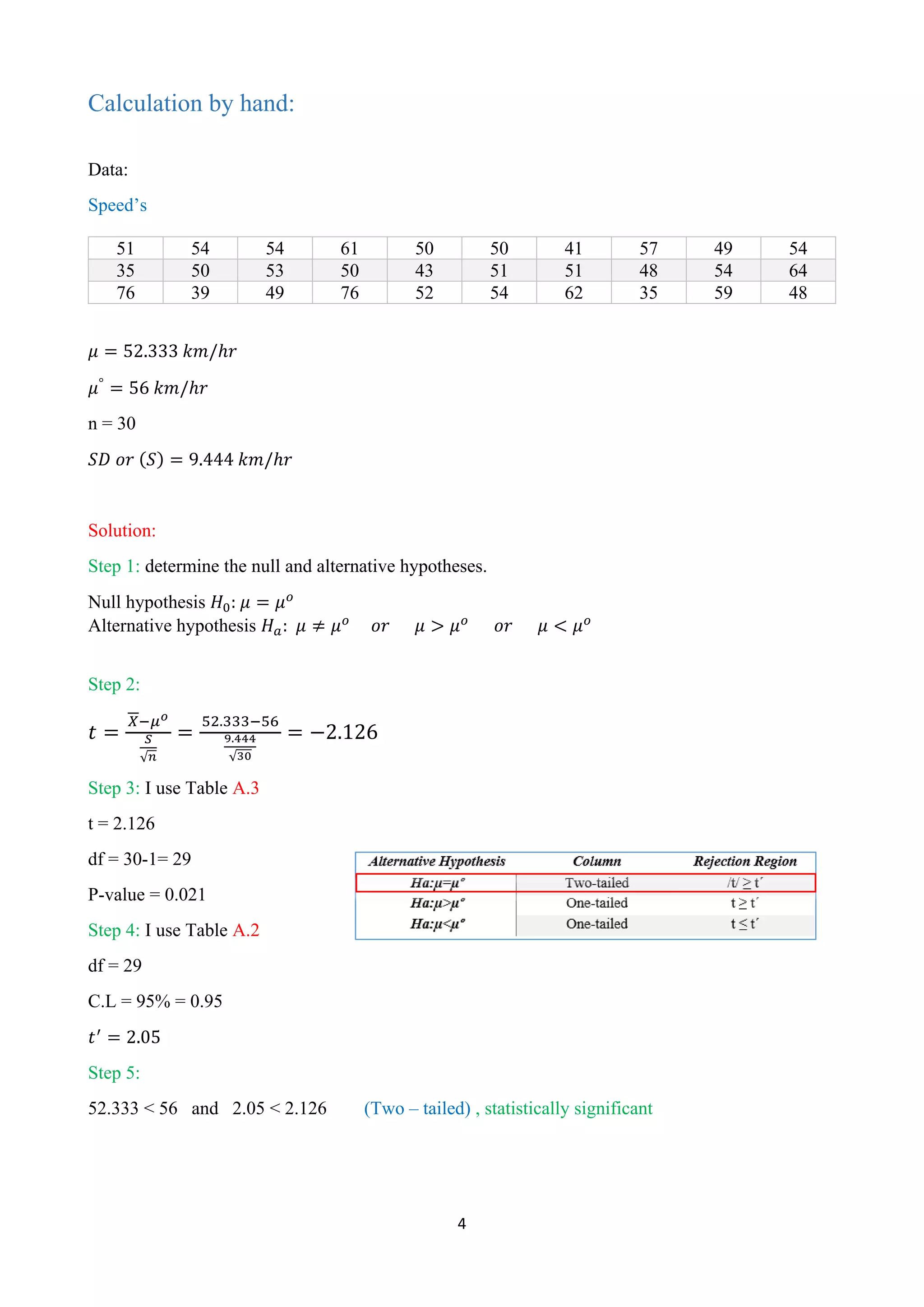
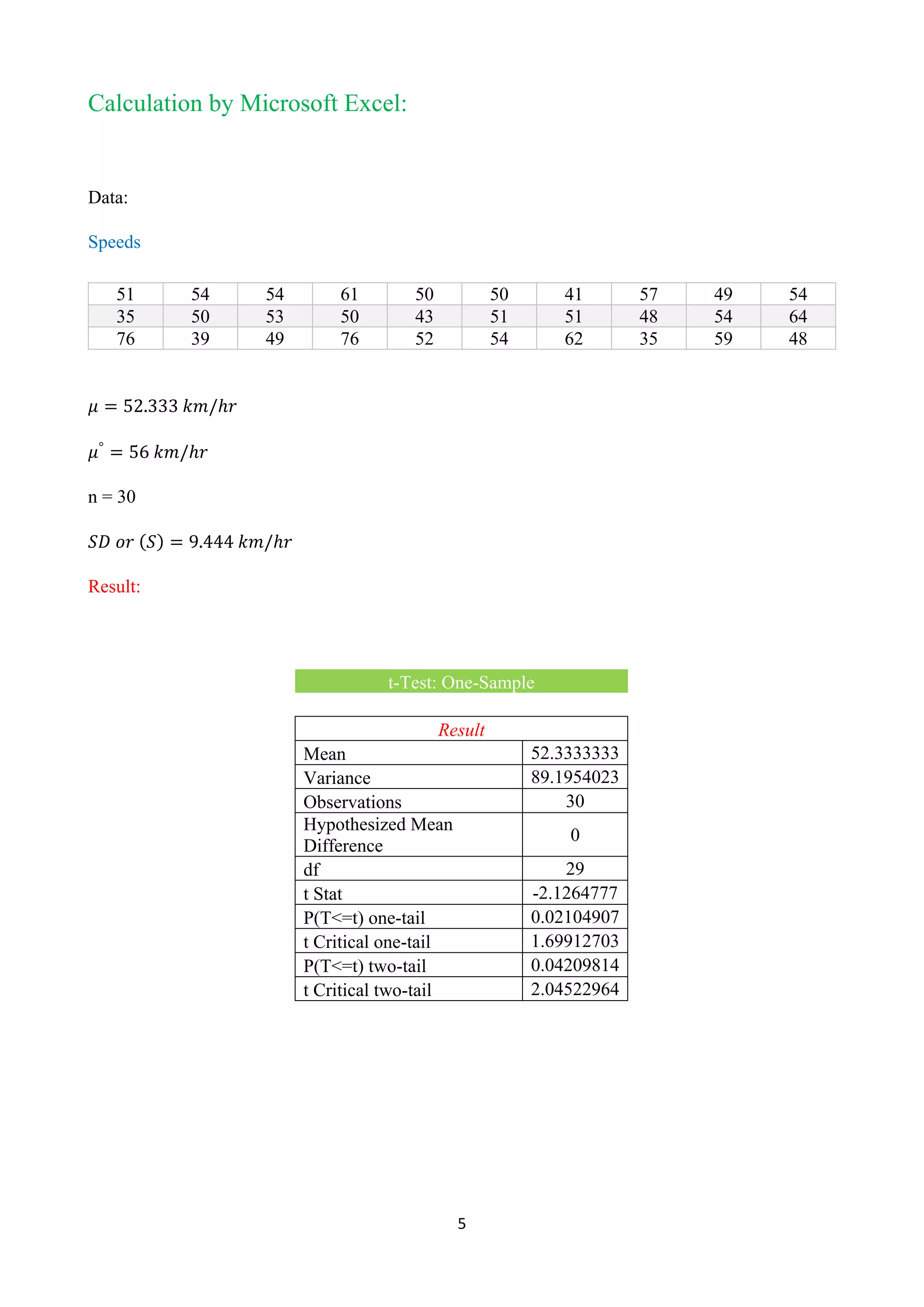
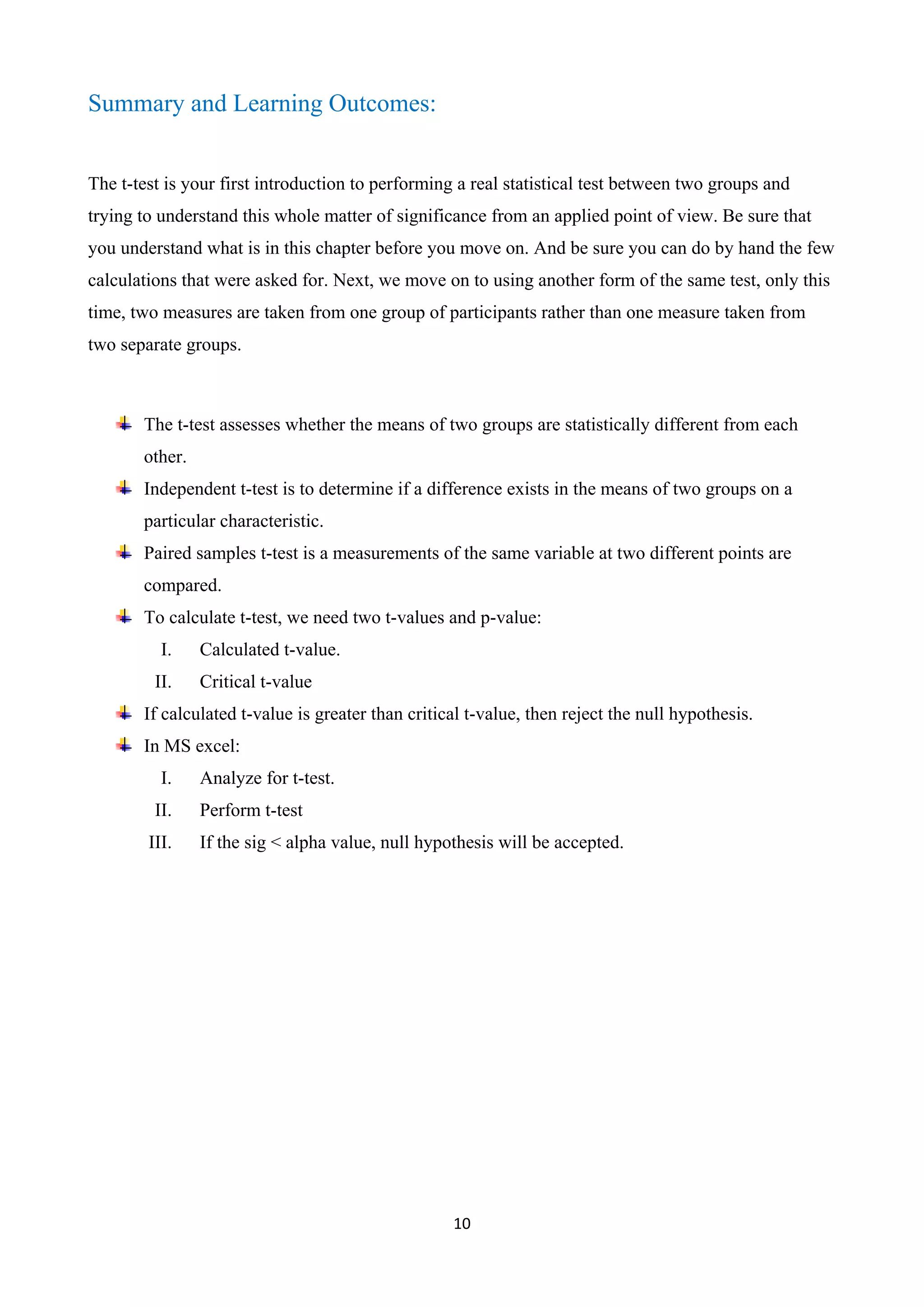
Discussion:
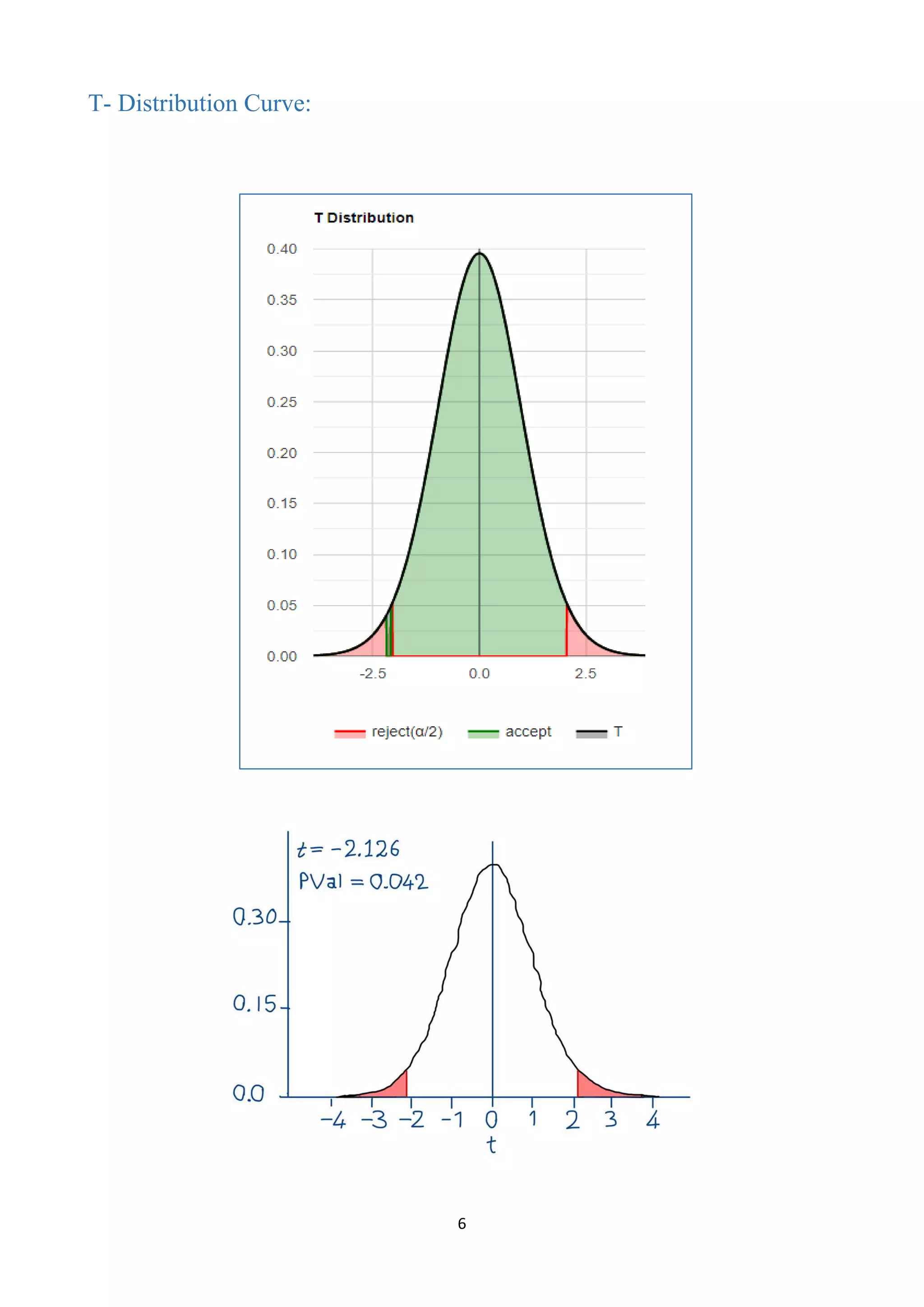
One sample t-test, using T distribution (DF=29) (two-tailed) (validation)
Since p-value < α, H0 is rejected.
The average of Speed's population is considered to be not equal to the μ0.
In other words, the difference between the average of the Speed and μ0 is big enough to be
statistically significant.
p-value equals 0.0420981, ( p( x ≤ T ) = 0.0210491 ). This means that the chance of type1 error
(rejecting a correct H0) is small: 0.04210 (4.21%).
The smaller the p-value the more it supports Ha.
The test statistic T equals -2.126478, is not in the 95% critical value accepted range: [-2.0452 :
2.0452].
x=52.33, is not in the 95% accepted range: [52.4700 : 59.5300].
The statistic S' equals 1.724 .
The observed standardized effect size is medium (0.39). That indicates that the magnitude of the
difference between the average and μ0 is medium.

9. 9
Summary and Learning Outcomes:
Step 1: Determine the null and alternative hypotheses.
where the format of the alternative hypothesis depends on the research question
of interest and must be decided before looking at the data.
Step 2: Summarize the data into an appropriate test statistic after first verifying
that necessary data conditions are met.
If n is large, or if there are no extreme outliers or skewness, compute
Step 3: Find the p-value by comparing the test statistic to the possibilities
expected if the null hypothesis were true.
Using the t-distribution with df 5 n 2 1, the p-value is the area in the tail(s)
beyond the test statistic t, as follows:
These areas can be found using statistical software, or a p-value range can be
found using Table A.3 in the Appendix.
Step 4: Decide whether the result is statistically significant based on the p-value.
Step 5: Report the conclusion in the context of the situation.
The notation t* is used for the multiplier in a confidence interval as well
as for the critical value in a rejection region. Values of t* are found in Table A.2.

10. 10
Summary and Learning Outcomes:
The t-test is your first introduction to performing a real statistical test between two groups and
trying to understand this whole matter of significance from an applied point of view. Be sure that
you understand what is in this chapter before you move on. And be sure you can do by hand the few
calculations that were asked for. Next, we move on to using another form of the same test, only this
time, two measures are taken from one group of participants rather than one measure taken from
two separate groups.
The t-test assesses whether the means of two groups are statistically different from each
other.
Independent t-test is to determine if a difference exists in the means of two groups on a
particular characteristic.
Paired samples t-test is a measurements of the same variable at two different points are
compared.
To calculate t-test, we need two t-values and p-value:
I. Calculated t-value.
II. Critical t-value
If calculated t-value is greater than critical t-value, then reject the null hypothesis.
In MS excel:
I. Analyze for t-test.
II. Perform t-test
III. If the sig < alpha value, null hypothesis will be accepted.

11. 11
Reference:
1-Mind on Statistics 5th ed Jessica M. Utts University of California, Irvine Robert F. Heckard
Pennsylvania State University.
2-Applied Statistics and Probability for Engineers Sixth Edition Douglas C. Montgomery Arizona
State University George C. Runger Arizona State University.
3-Basic Statistics for Business & Economics Fifth Edition Douglas A. Lind Coastal Carolina
University and The University of Toledo William C. Marchal The University of Toledo SamuelA.
Wathen Coastal Carolina University.
4-Excel 2016 for Engineering Statistics A Guide to Solving Practical Problems /Thomas J. Quirk.
5- statistics for people who hate statistics 6th
ed —Professor Valarie Janesick Professor of
Educational Leadership University of South Florida.
6- Engineering Statistics 2019-2020 lecturer. Dilveen H. Omar.