Download to read offline
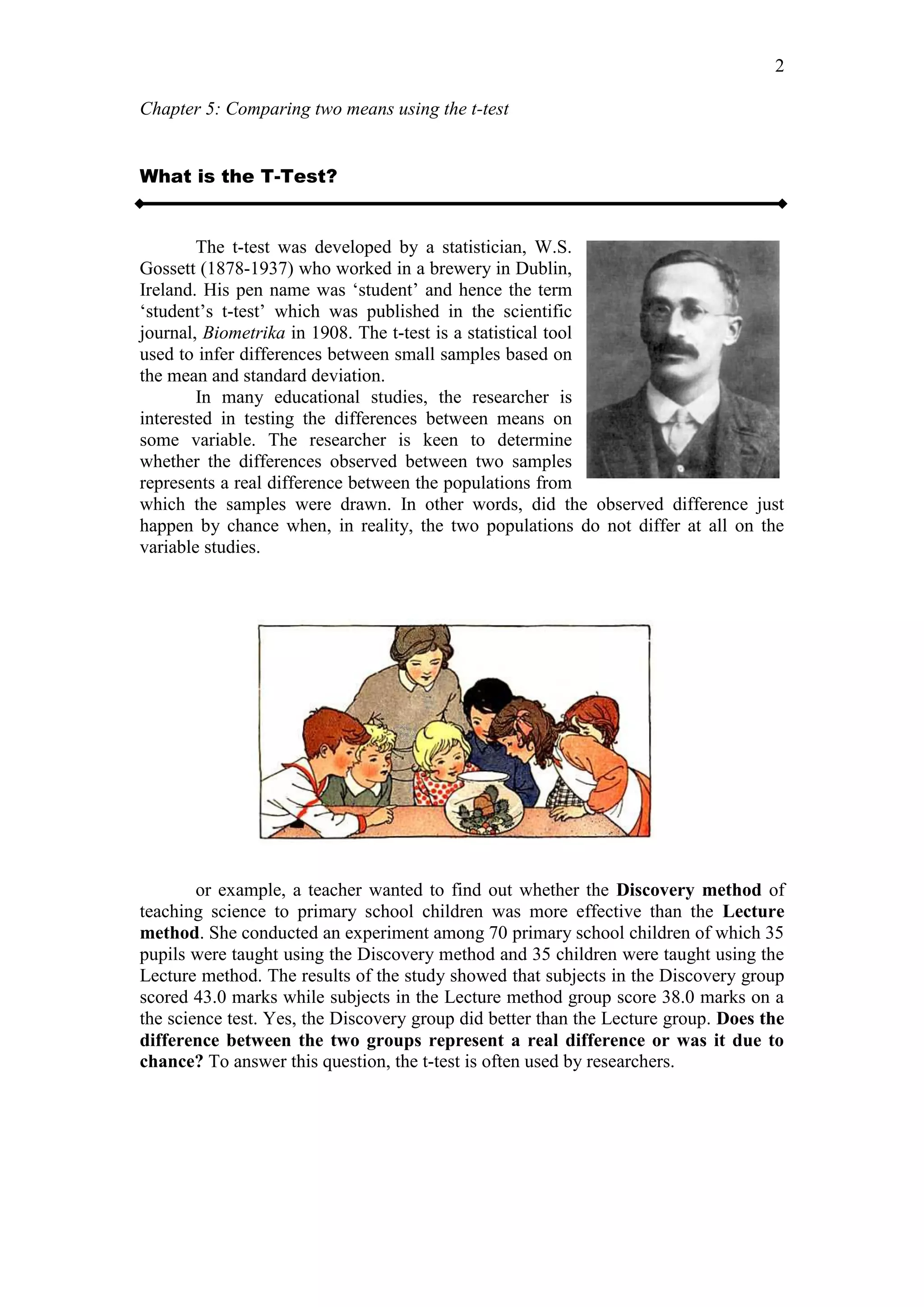
![Chapter 5: Comparing two means using the t-test
10
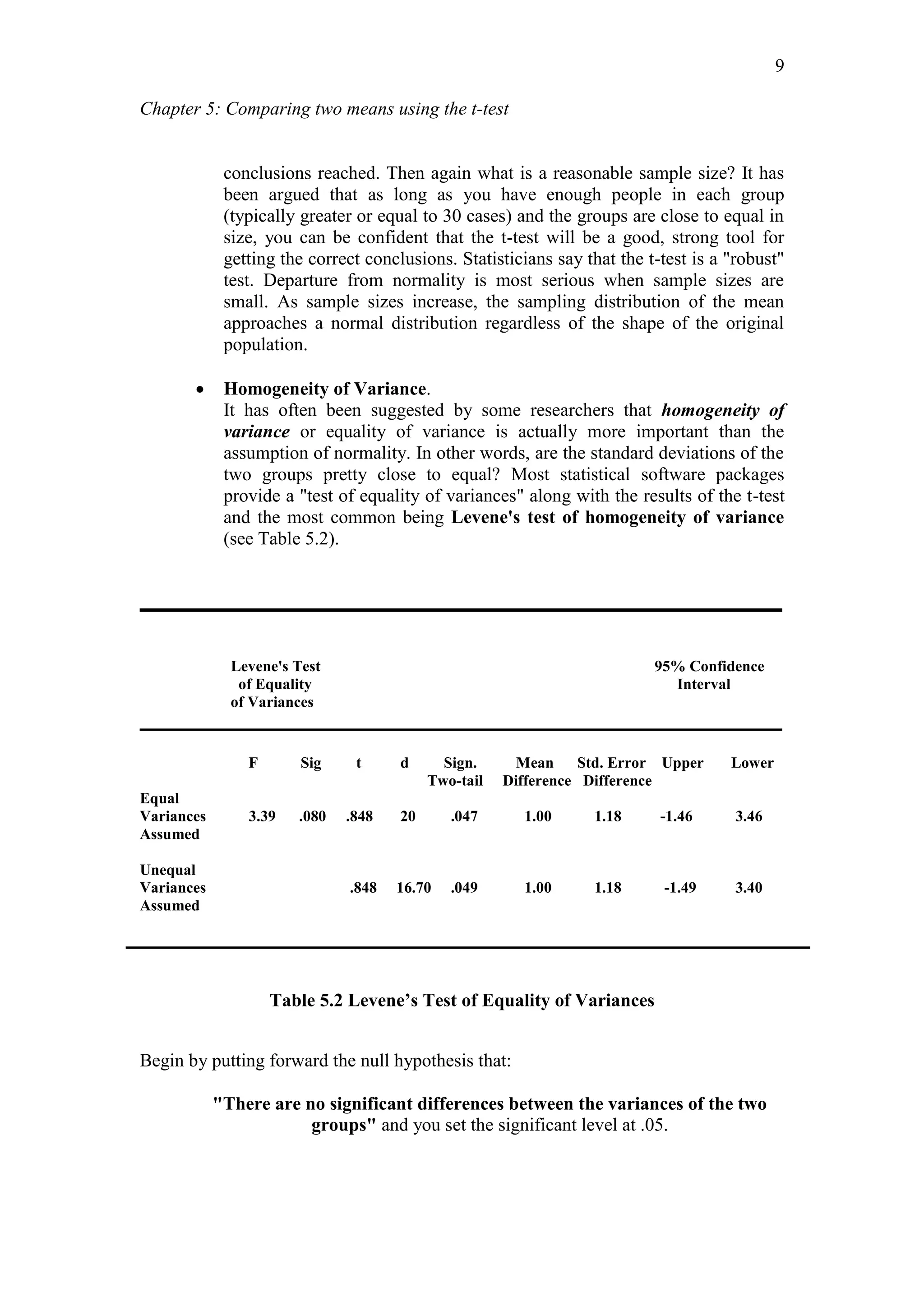
If the Levene statistic is significant, i.e. LESS than .05 level (p < .05), then the null
hypothesis is:
REJECTED and one accepts the alternative hypothesis and conclude that
the VARIANCES ARE UNEQUAL. [The unequal variances in the SPSS
output is used]
If the Levene statistic is not significant, i.e. MORE than .05 level (p > .05),
then you DO NOT REJECT (or Accept) the null hypothesis and conclude
that the VARIANCES ARE EQUAL. [The equal variances in the SPSS
output is used]
The Levene test is robust in the face of departures from normality. The Levene's test
is based on deviations from the group mean.
SPSS provides two options'; i.e. "homogeneity of variance assumed" and
"homogeneity of variance not assumed" (see Table below).
The Levene test is more robust in the face of non-normality than more
traditional tests like Bartlett's test.
Let’s examine an EXAMPLE:
In the CoPs Project, an Inductive Reasoning scale consisting of 11 items was
administered to 946 eighteen year. One of the research questions put forward is:
"Is there a significant difference between in inductive reasoning between
male and female subjects"?
To establish the statistical significance of the means of these two groups, the t-
test was used. Using SPSS.
LEARNING ACTIVITY
Refer to the table above. Based on the Levene’s Test of
Homogeneity of variance, what is your conclusion. Explain.](https://image.slidesharecdn.com/chapter5t-test-170406172651/75/Chapter-5-t-test-10-2048.jpg)
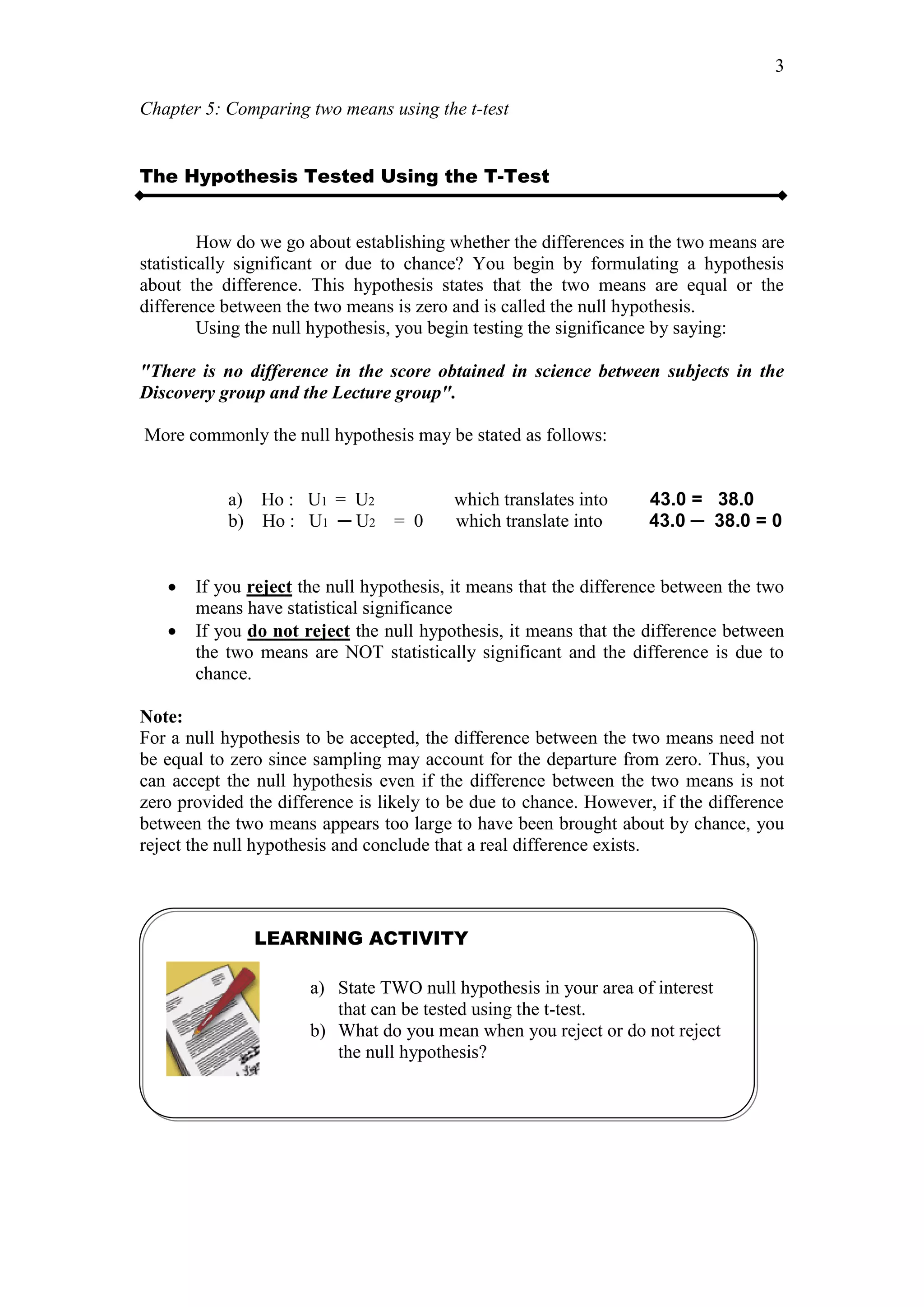
![Chapter 5: Comparing two means using the t-test
11
THE SPSS STEPS to answer the Research Question.
SPSS OUTPUTS:
Output #1:
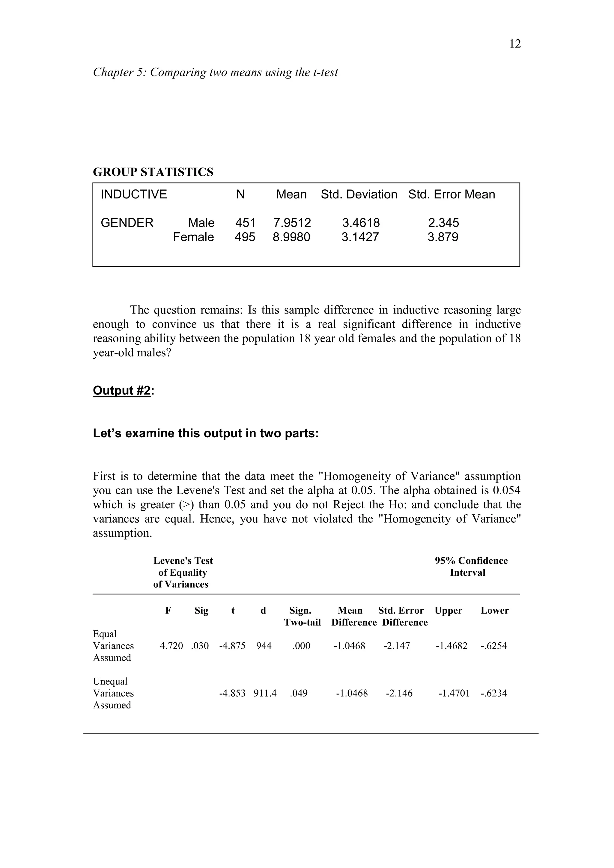
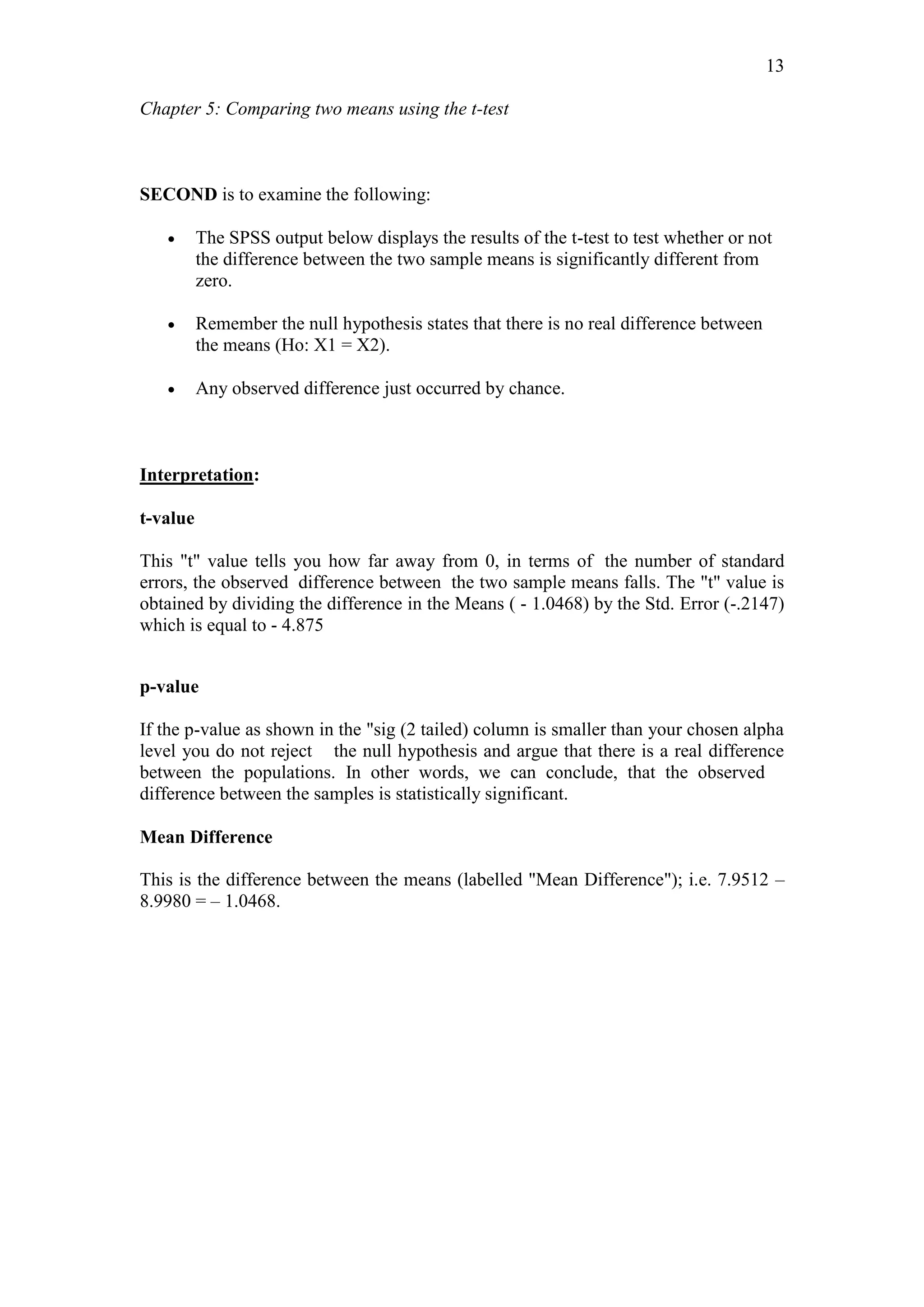
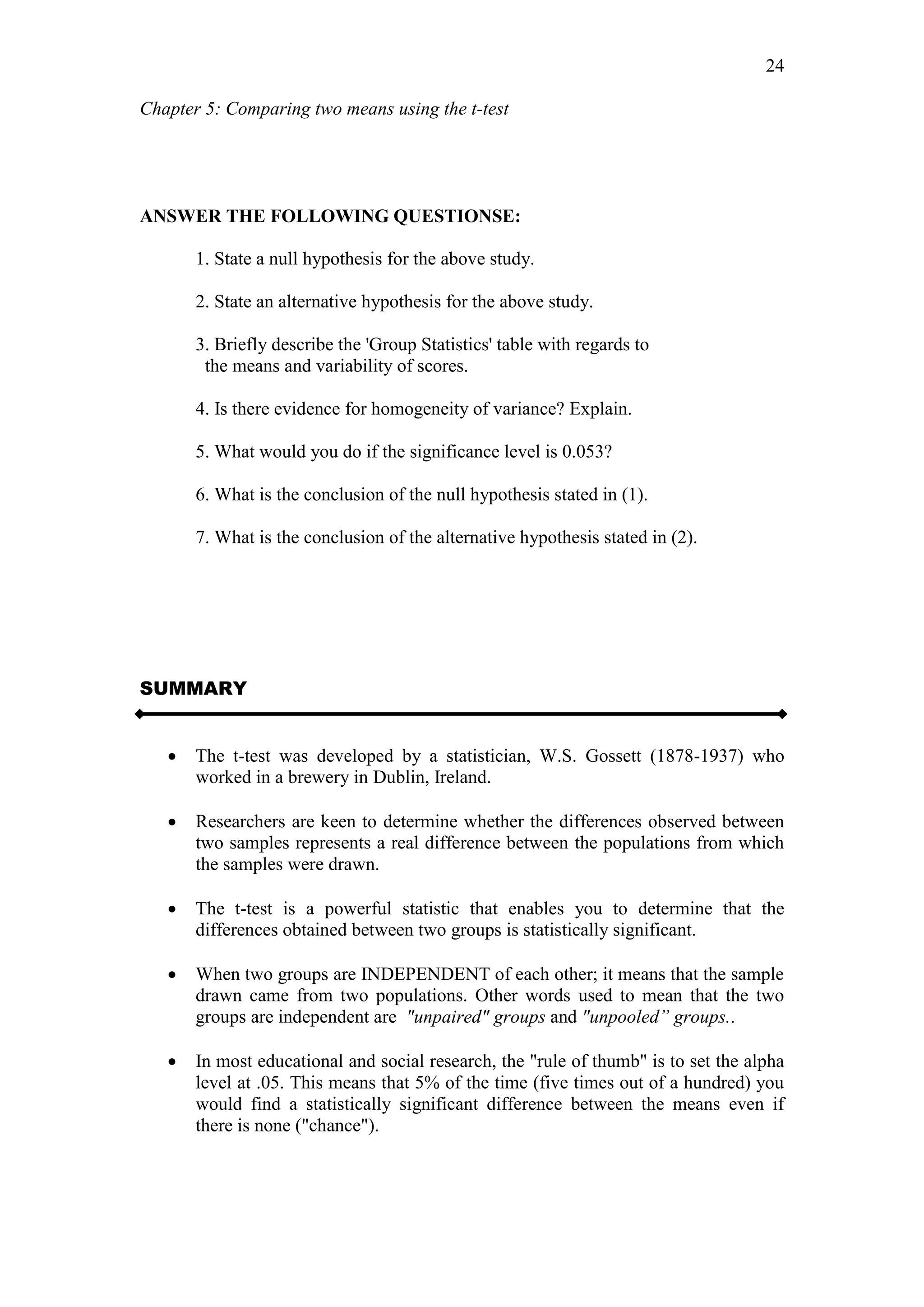
The ‘Group statistics’ table above reports that the mean values on the variable
(inductive reasoning) for the two different groups (males and females). Here, we see
that the 495 females in the sample scored 8.99 while the 451 males had a mean score
of 7.95 on inductive reasoning. The standard deviation for the males is 3.46 while
that for the females is 3.14. The scores for the females are less dispersed compared to
the males.
SPSS PROCEDURES for the independent groups t-test:
1. Select the Analyze menu.
2. Click on Compare Means and then Independent-
Samples T Test ....to open the Independent Samples
T Test dialogue box.
3. Select the test variable(s). [i.e. Inductive Reasoning] and
then click on the button to move the variables into
the Test Variables(s): box
4. Select the grouping variables [i.e. gender] and click on
the button to move the variable into the Grouping Variable:
box
5. Click on the Define Groups ....command pushbutton to
open the Define Groups sub-dialogue box.
6. In the Group 1: box, type the lowest value for the variable
[i.e. 1 for 'males'], then tab. Enter the second value for the
variables [i.e. 2 for 'females'] in the Group 2: box.
7. Click on Continue and then OK.](https://image.slidesharecdn.com/chapter5t-test-170406172651/75/Chapter-5-t-test-11-2048.jpg)
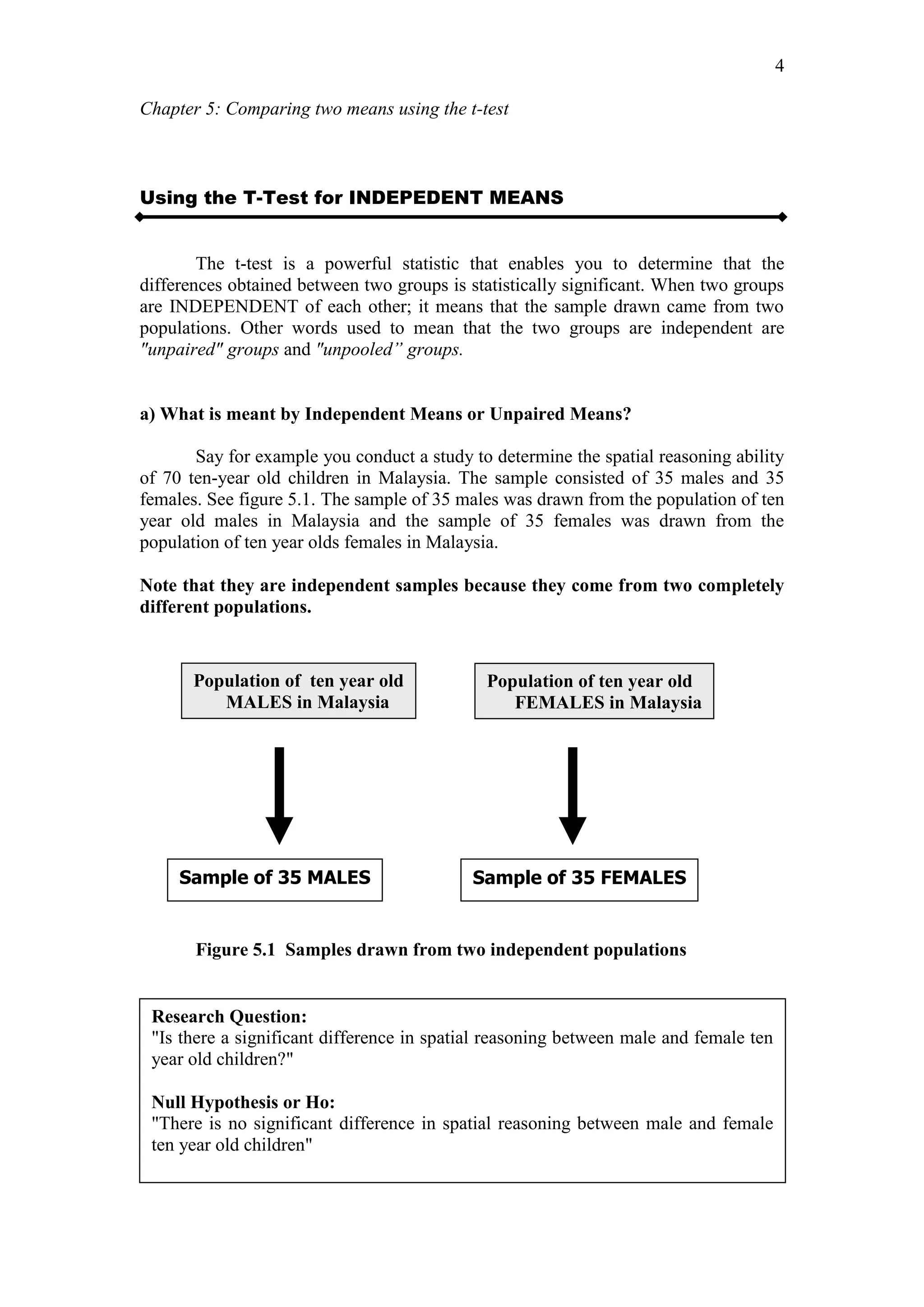
![Chapter 5: Comparing two means using the t-test
17
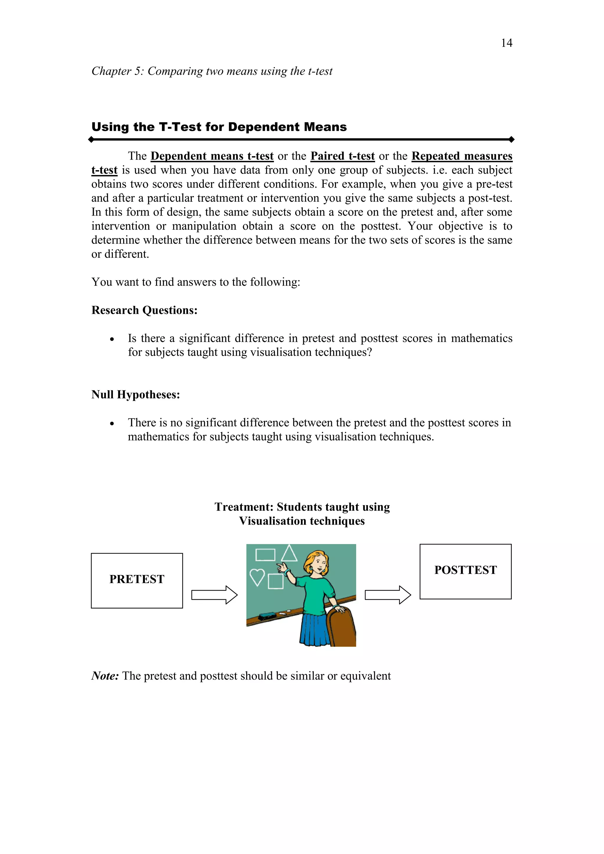
Excerpt of the Table of Critical Values for Student's t-test
Tailed
Two 0.100 0.050 0.025 0.010 0.005
One 0.200 0.100 0.050 0.020 0.010
df
9 1.383 1.833 2.262 2.821 3.250
10 1.372 1.812 2.228 2.764 3.169
11 1.363 1.796 2.201 2.718 3.106
12 1.356 1.782 2.179 2.681 3.055
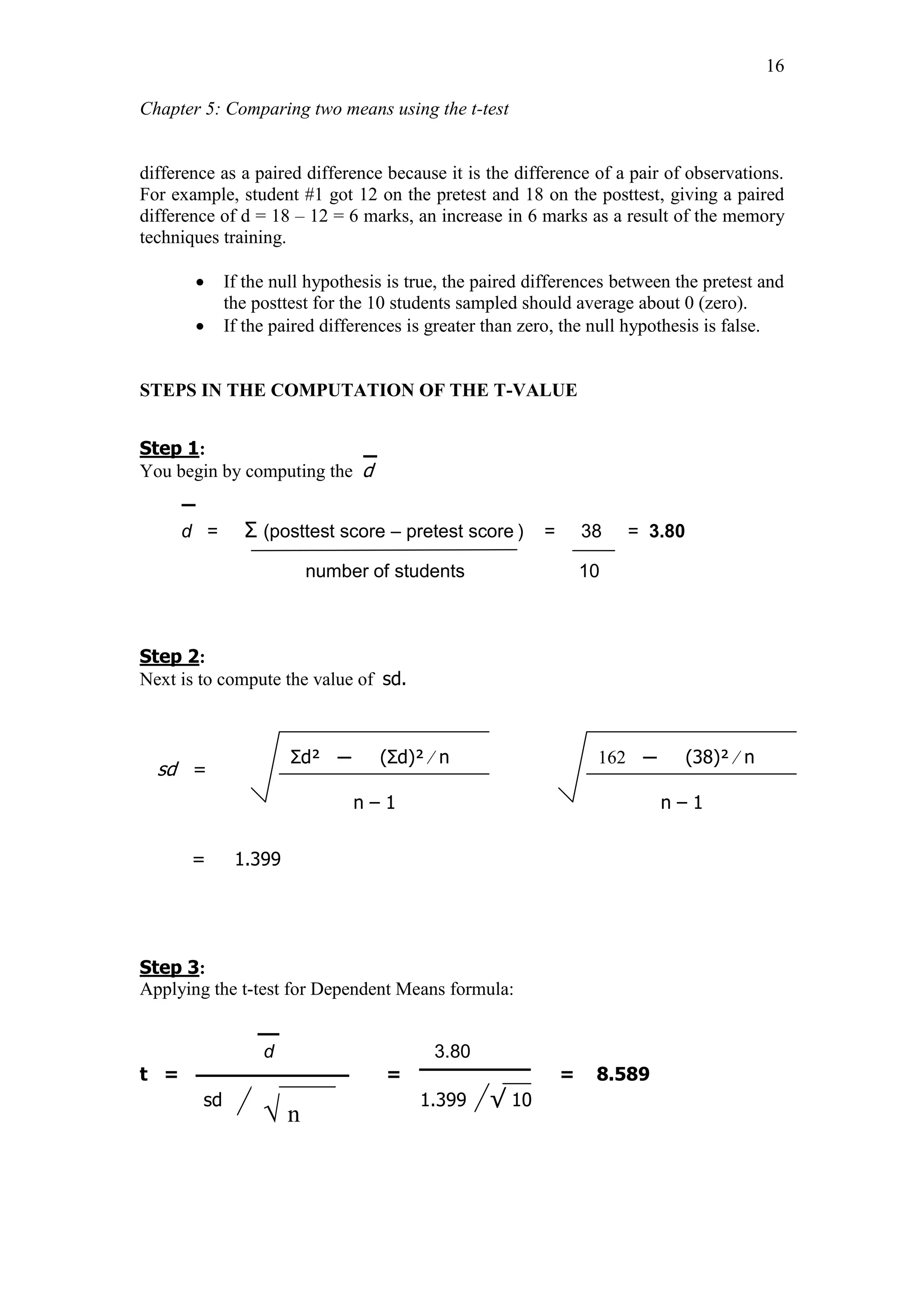
Step 4:
Having computed the t-value (which is 8.589) you look up the t-value in The Table
of Critical Values for Student's t-test or The Table of Significance which tells us
whether the ratio is large enough to say that the difference between the groups is
significant. In other words the difference observed is not likely due to chance or
sampling error.
Alpha Level:
The researcher set the alpha level at 0.05. This means that 5% of the time (five out of
a hundred) you would find a statistically significant difference between the means
even if there is none ("chance").
Degrees of Freedom:
The t-test also requires that we determine the degrees of freedom (df) for the test. In
the t-test, the degrees of freedom is the sum of the subjects or persons which is 10
minus 1 = 9. Given the alpha level, the df, and the t-value, you look up in the Table
(available as an appendix in the back of most statistics texts) to determine whether the
t-value is large enough to be significant.
Step 5:
The t-value obtained is 8.589 which is greater than the critical value shown which is
1.833 (one tailed). Hence, the null hypothesis [Ho:] is Rejected and Ha: is accepted](https://image.slidesharecdn.com/chapter5t-test-170406172651/75/Chapter-5-t-test-17-2048.jpg)
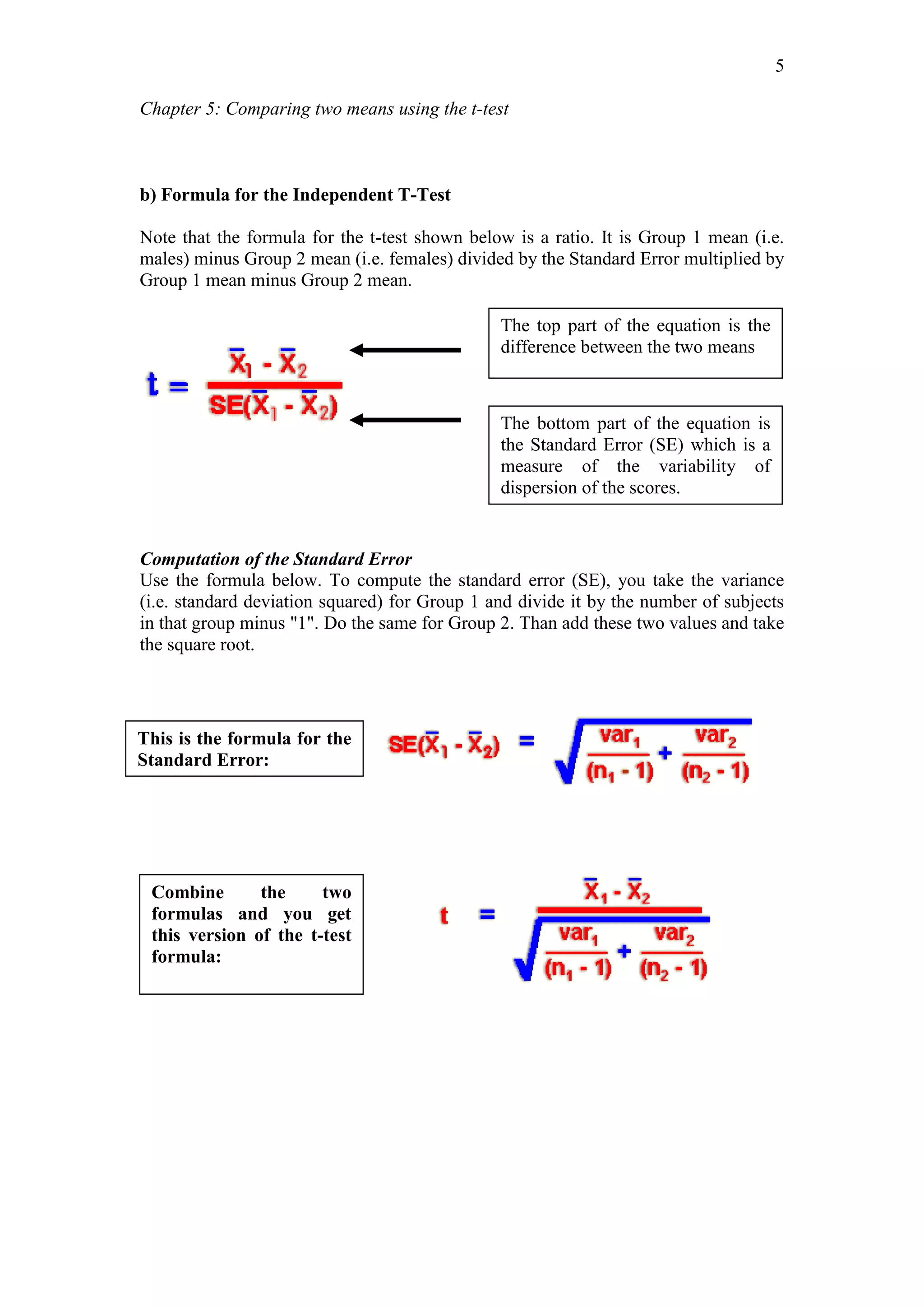
![Chapter 5: Comparing two means using the t-test
19
Data was collected from the same group of subjects on both conditions and
each subject obtains a score on the pretest, and after the treatment (or intervention or
manipulation), a score on the posttest.
Ho: U1 = U2 or Ha: U1 = U2
You will notice that the syntax for the Independent Groups t-test is different from that
of the Dependent groups t-test. In the case of the Independent Groups t-test you have
a grouping variable so you can distinguish between Group 1 and Group 2 whereas
this is not found with the Dependent groups t -test.
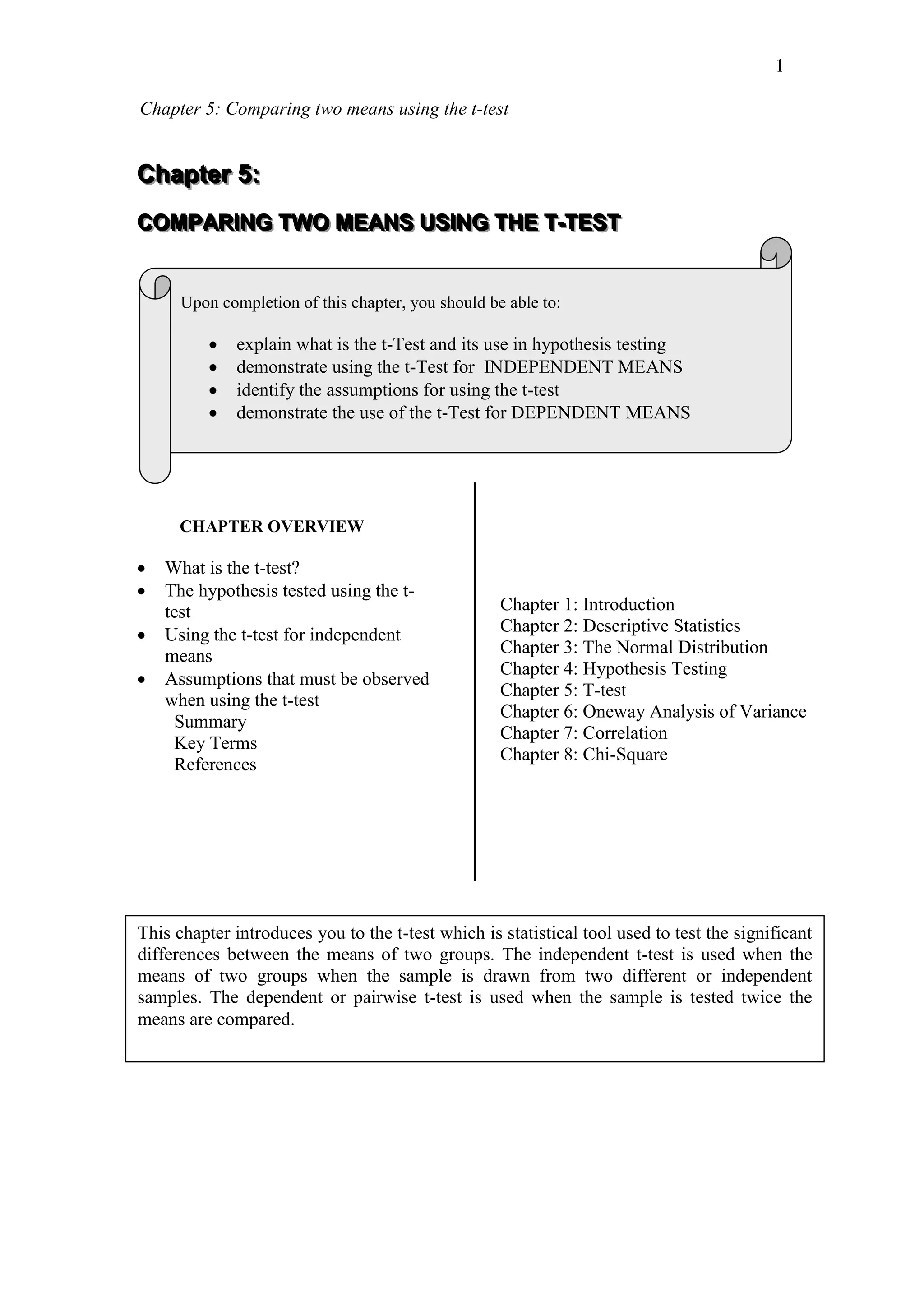
The following are the SPSS OUTPUTS:
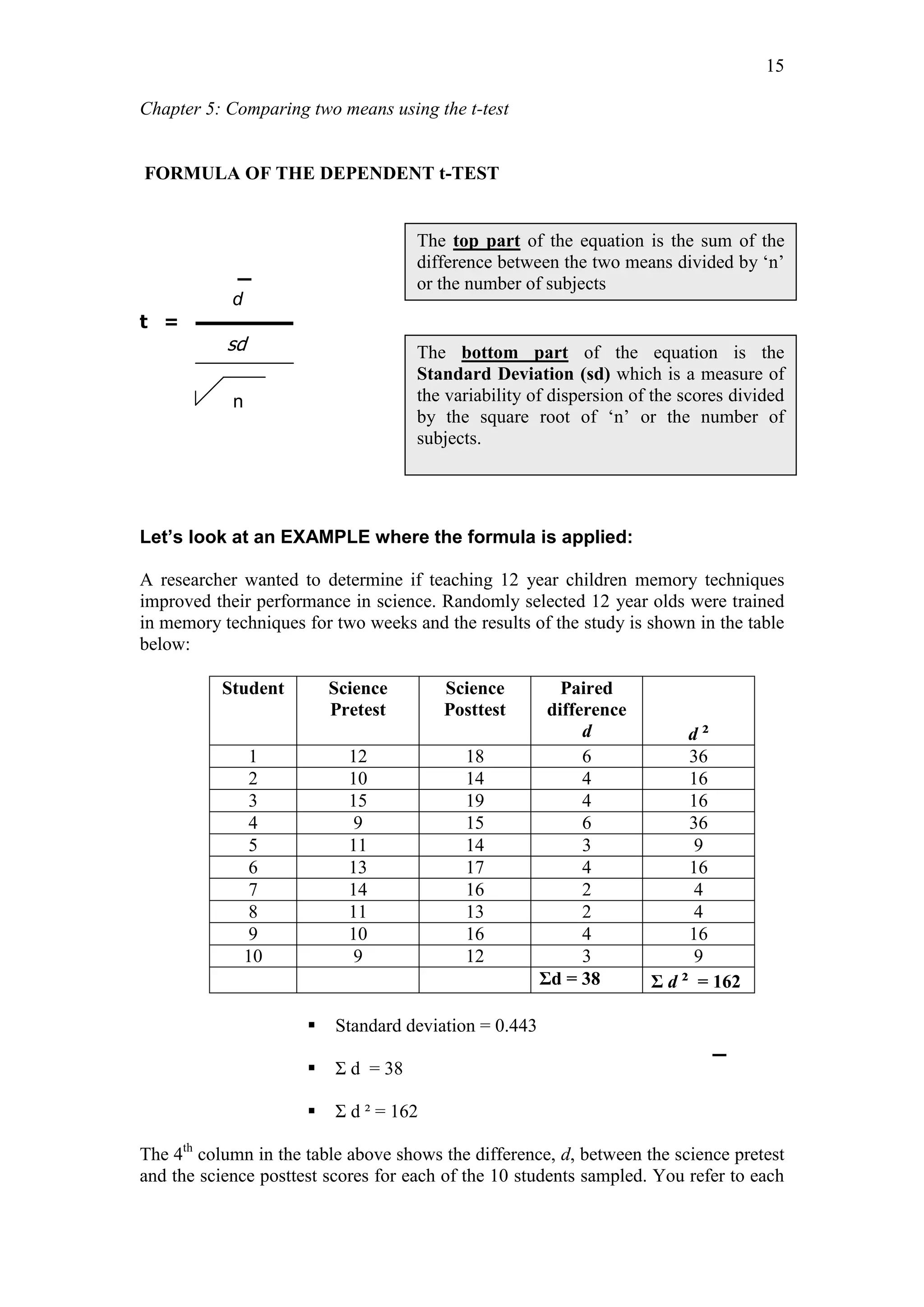
Paired Sample Statistics
HISTORY TEST N Mean Std. Deviation Std. Error Mean
Pair Pretest 40 43.15 12.97 2.05
Posttest 40 63.98 13.16 2.08
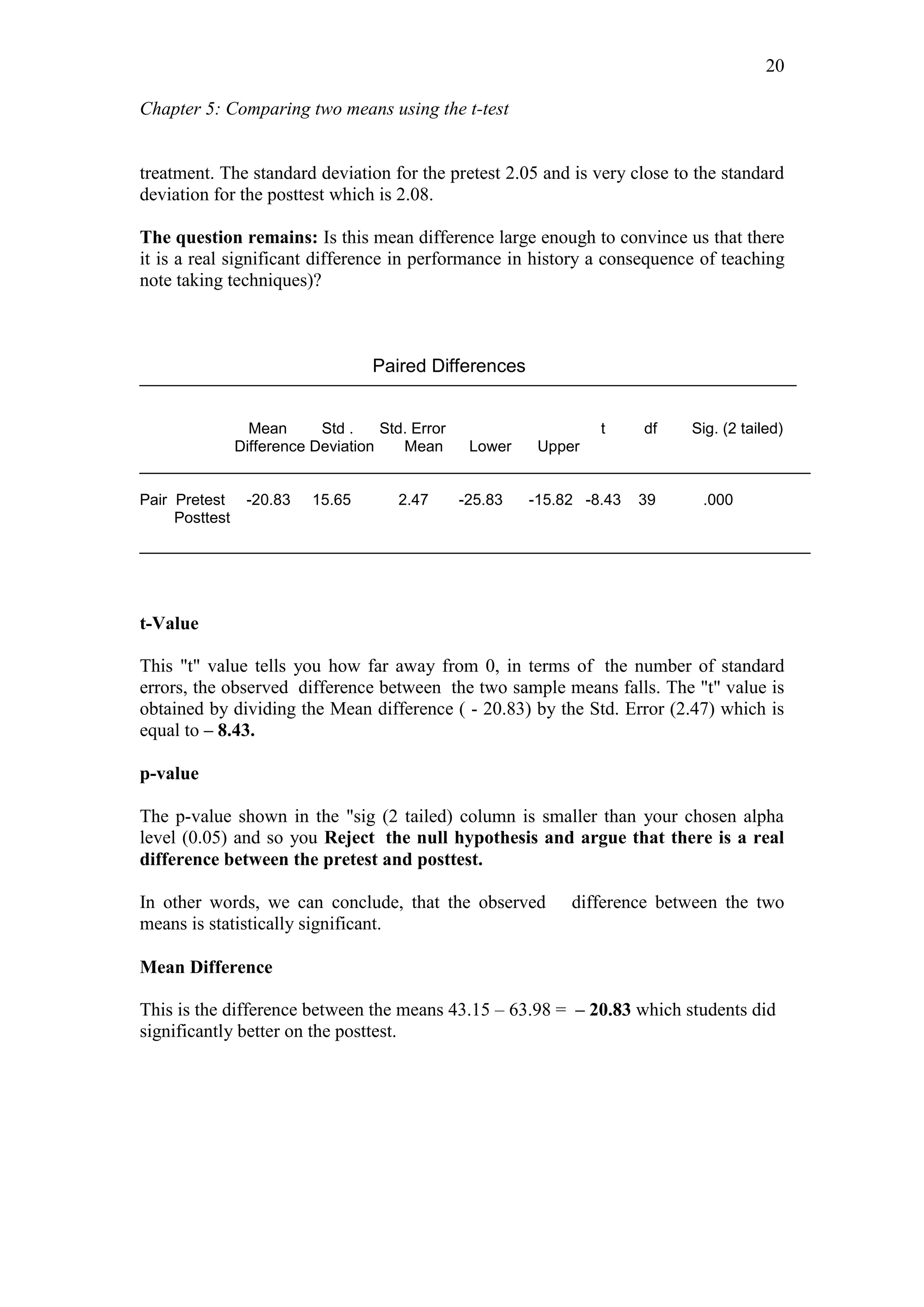
The ‘Paired sample statistics’ table above reports that the mean values on the variable
(history test) for the pretest and posttest. The posttest mean is higher (63.98) than the
posttest mean (43.15) indicating improved performance in the history test after the
SPSS PROCEDURES for the dependent groups t-test:
1. Select the Analyze menu.
2. Click on Compare Means and then Paired-Samples T Test
....to open the Paired-Sample T Test dialogue box.
3. Select the test variable(s). [i.e. History Test] and
then press the button to move the variables into
the Paired Variables: box
4. Click on Continue and then OK.](https://image.slidesharecdn.com/chapter5t-test-170406172651/75/Chapter-5-t-test-19-2048.jpg)


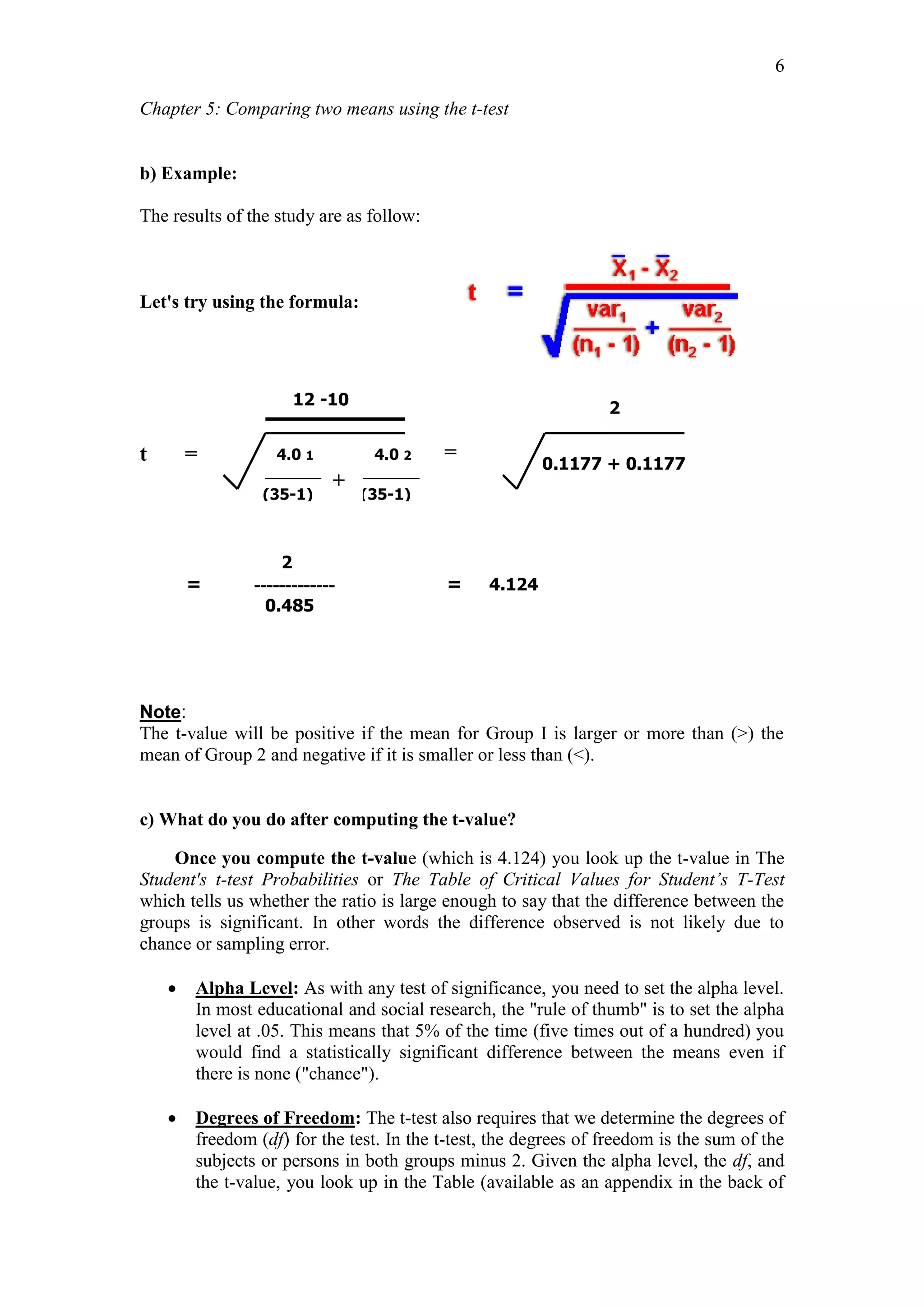
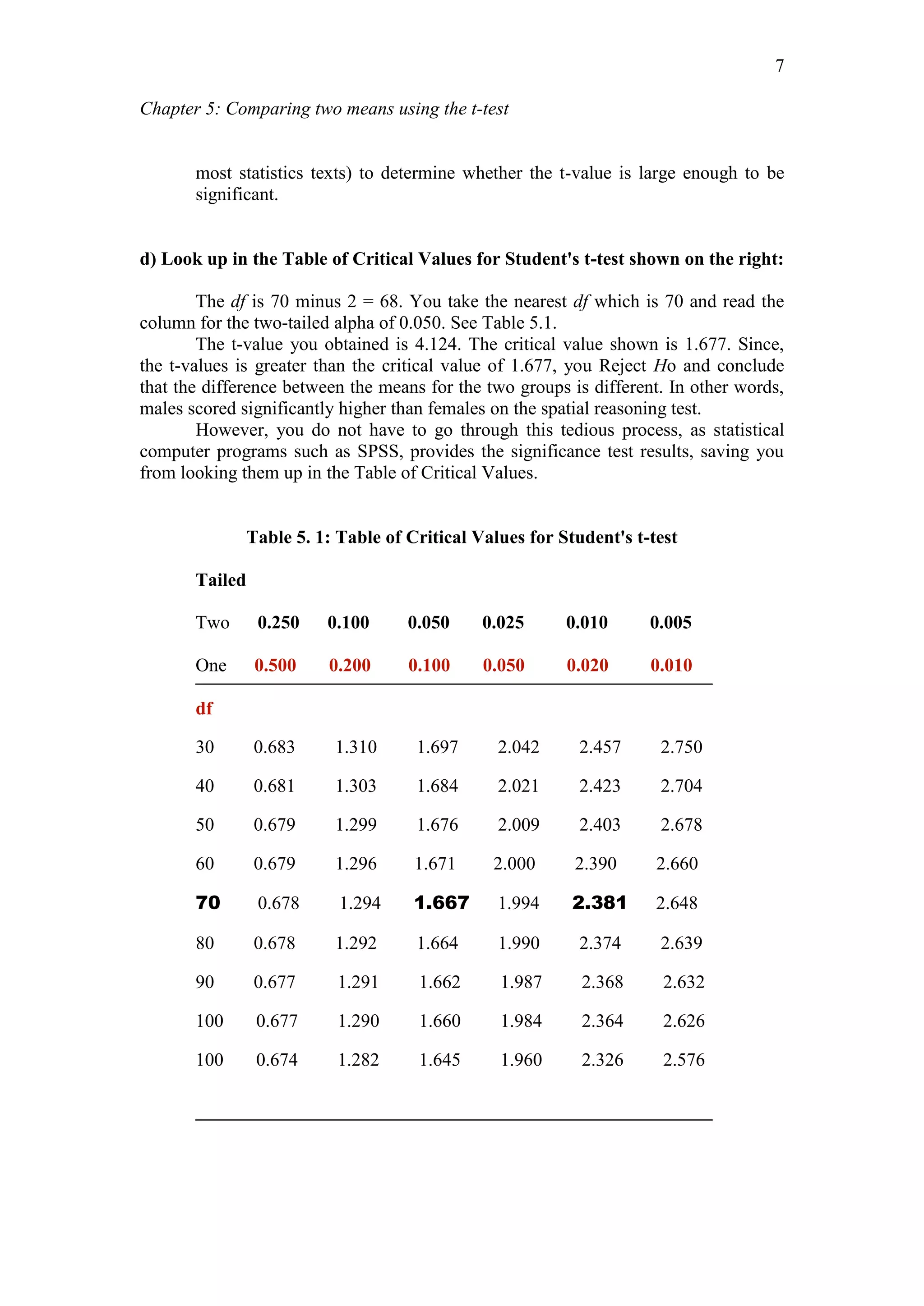
This chapter introduces the t-test, a statistical tool used to test for significant differences between the means of two groups. It discusses the independent t-test for comparing means of two independent samples, and the dependent or paired t-test for comparing means of the same sample tested twice. The chapter covers the assumptions of the t-test, how to formulate hypotheses, compute t-values, and interpret results based on critical values. Key aspects include the formula for computing the t-statistic and standard error, conducting significance tests using t-distribution tables, and checking assumptions such as normality and homogeneity of variance.