Downloaded 40 times

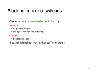
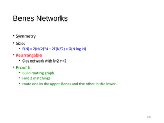
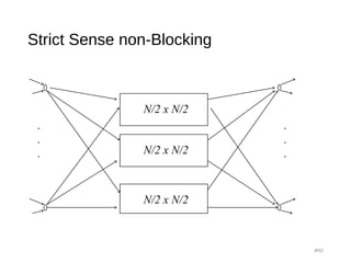
![Clos Network - strict sense non-blocking
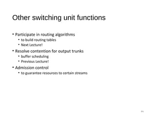
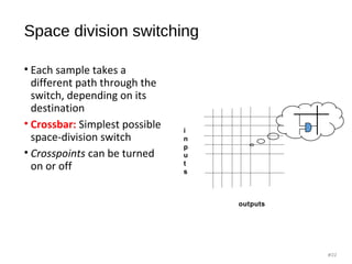
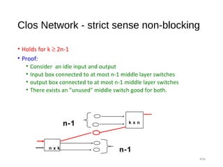
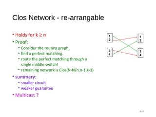
• Holds for k ≥ 2n-1
• Proof Methodology:
• Recall: IF [A,B ⊆ S and |A|+|B| > |S|] then A∩ B≠Ø
• S= The k middle switches
• A = middle switches reachable from the inputs
• B = middle switches reachable from the outputs
• Our case:
• |S|=k
• |A| ≥ k-(n-1)
• |B| ≥ k-(n-1)
#35](https://image.slidesharecdn.com/switchingunits-170203123341/85/Switching-units-34-320.jpg)
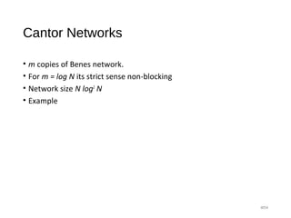
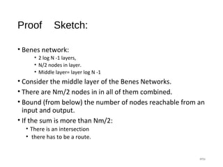
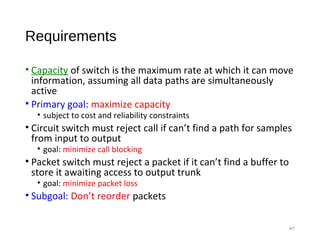
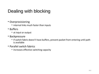
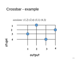
![Proof Sketch:
• Let A(k) = number of nodes reachable at level k.
• A(0)=m
• A(1)= 2A(0)-1
• A(2)=2A(1)-2
• A(k)=2A(k-1) - 2k-1
= 2k
A(0) - k 2k-1
• A(log N -1) = Nm/2 - (log N -1) N/4
• Need that: 2A(log N -1) > Nm/2.
• 2[Nm/2 - (log N -1) N/4] > Nm/2.
• Hold for m> log N-1.
#57](https://image.slidesharecdn.com/switchingunits-170203123341/85/Switching-units-56-320.jpg)

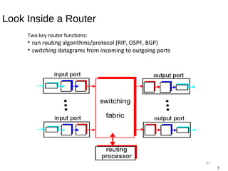
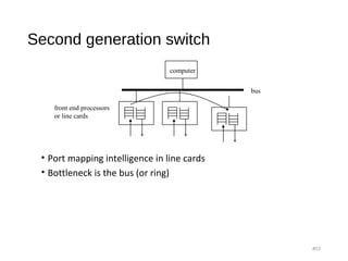
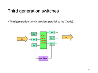
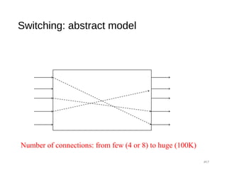
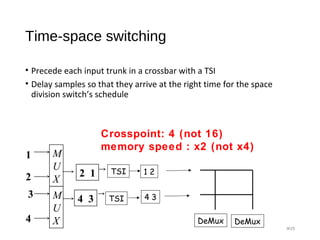
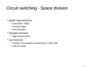
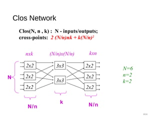
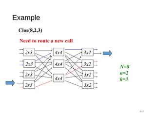
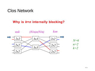
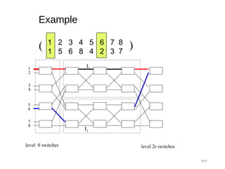
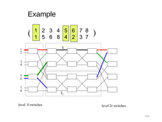
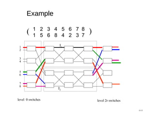
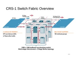
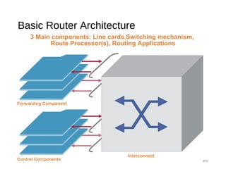
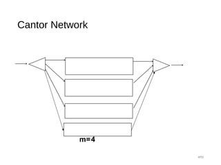
The document provides an overview of various switching mechanisms including telephone switches, routers, and packet switches, explaining their functionalities and types such as circuit- and connection-oriented switching. It discusses the importance of internal switching mechanisms, blocking issues in packet switching, and methods to handle such blockages along with the evolution and generations of packet switches. Additionally, the document delves into specific switching architectures like Clos networks, Benes networks, and their complexity, scalability, and non-blocking properties.


![[Deck] What's New in Spark-Iceberg Integration via DSV2.pptx](https://cdn.slidesharecdn.com/ss_thumbnails/deckwhatsnewinspark-icebergintegrationviadsv2-260210005337-25955b12-thumbnail.jpg?width=640&height=640&fit=bounds)


