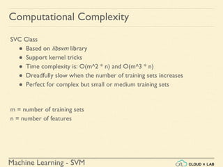
Downloaded 89 times


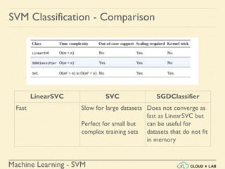
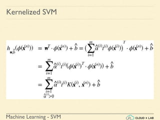
![Machine Learning - SVM
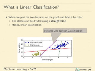
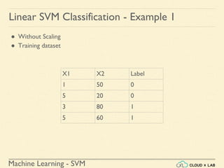
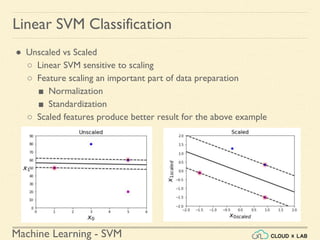
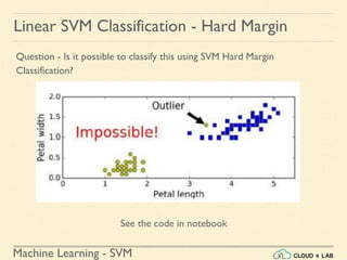
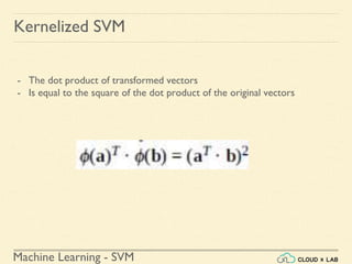
Linear SVM Classification - Example 1
● Model the classifier, plot the points and the classifier
>>> Xs = np.array([[1, 50], [5, 20], [3, 80], [5,
60]]).astype(np.float64)
>>> ys = np.array([0, 0, 1, 1])
>>> svm_clf = SVC(kernel="linear", C=100)
>>> svm_clf.fit(Xs, ys)
>>> plt.plot(Xs[:, 0][ys==1], Xs[:, 1][ys==1], "bo")
>>> plt.plot(Xs[:, 0][ys==0], Xs[:, 1][ys==0], "ms")
>>> plot_svc_decision_boundary(svm_clf, 0, 6)
>>> plt.xlabel("$x_0$", fontsize=20)
>>> plt.ylabel("$x_1$ ", fontsize=20, rotation=0)
>>> plt.title("Unscaled", fontsize=16)
>>> plt.axis([0, 6, 0, 90])](https://image.slidesharecdn.com/5-180514114313/85/Support-Vector-Machines-36-320.jpg)
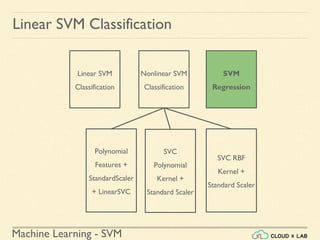
![Machine Learning Project
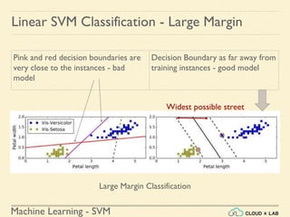
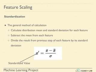
Feature Scaling
Min-max Scaling
● Also known as Normalization
● Normalized values are in the range of [0, 1]](https://image.slidesharecdn.com/5-180514114313/85/Support-Vector-Machines-42-320.jpg)
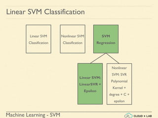
![Machine Learning Project
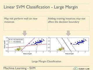
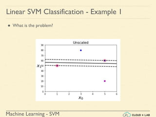
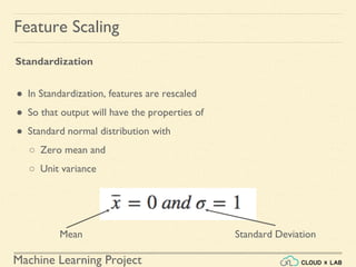
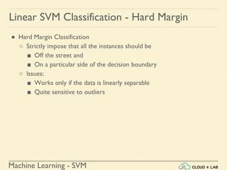
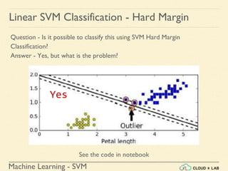
Feature Scaling
Min-max Scaling
● Also known as Normalization
● Normalized values are in the range of [0, 1]
Original Value
Normalized Value](https://image.slidesharecdn.com/5-180514114313/85/Support-Vector-Machines-43-320.jpg)
![Machine Learning Project
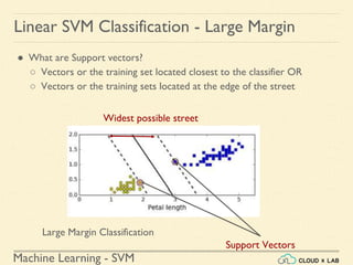
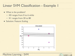
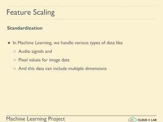
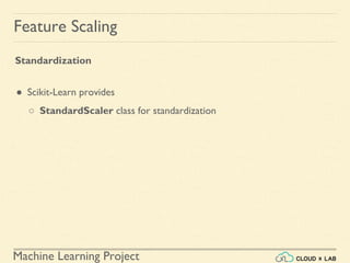
Feature Scaling
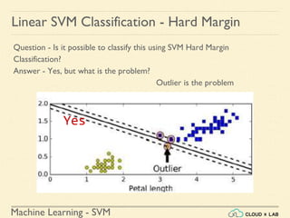
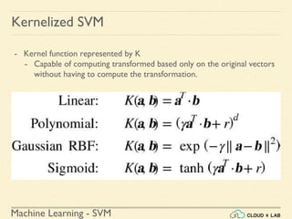
Min-max Scaling - Example
# Creating DataFrame first
>>> import pandas as pd
>>> s1 = pd.Series([1, 2, 3, 4, 5, 6], index=(range(6)))
>>> s2 = pd.Series([10, 9, 8, 7, 6, 5], index=(range(6)))
>>> df = pd.DataFrame(s1, columns=['s1'])
>>> df['s2'] = s2
>>> df](https://image.slidesharecdn.com/5-180514114313/85/Support-Vector-Machines-44-320.jpg)
![Machine Learning Project
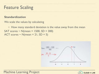
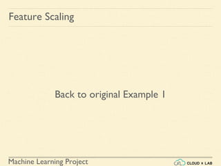
Feature Scaling
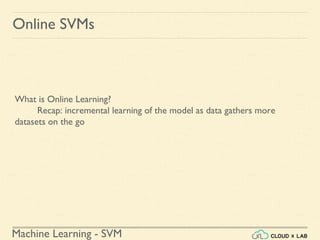
Min-max Scaling - Example
# Use Scikit-Learn minmax_scaling
>>> from mlxtend.preprocessing import minmax_scaling
>>> minmax_scaling(df, columns=['s1', 's2'])
Original Scaled (In range of
0 and 1)](https://image.slidesharecdn.com/5-180514114313/85/Support-Vector-Machines-45-320.jpg)
![Machine Learning Project
Feature Scaling
Which One to Use?
● Min-max scales in the range of [0,1]
● Standardization does not bound values to a specific range
○ It may be problem for some algorithms
○ Example- Neural networks expect an input value ranging from 0 to 1
● We’ll learn more use cases as we proceed in the course](https://image.slidesharecdn.com/5-180514114313/85/Support-Vector-Machines-51-320.jpg)
![Machine Learning - SVM
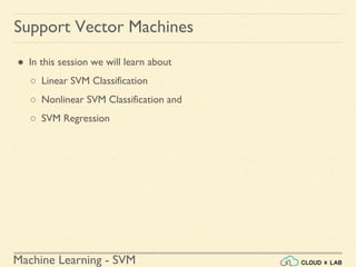
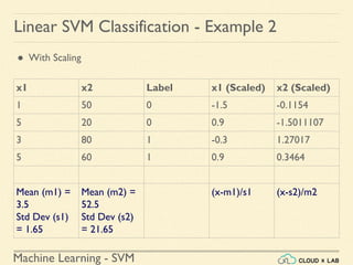
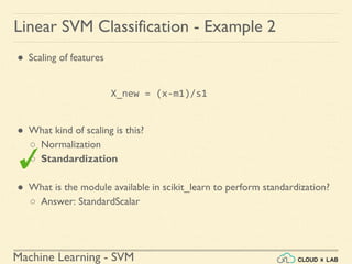
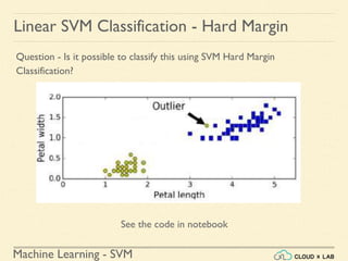
Linear SVM Classification - Example 2
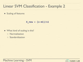
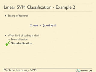
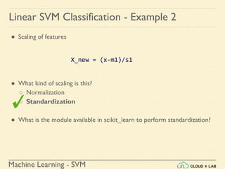
● Scaling the input training data
>>> from sklearn.preprocessing import StandardScaler
>>> scaler = StandardScaler()
>>> X_scaled = scaler.fit_transform(Xs)
>>> print(X_scaled)
[[-1.50755672 -0.11547005]
[ 0.90453403 -1.5011107 ]
[-0.30151134 1.27017059]
[ 0.90453403 0.34641016]]](https://image.slidesharecdn.com/5-180514114313/85/Support-Vector-Machines-58-320.jpg)
![Machine Learning - SVM
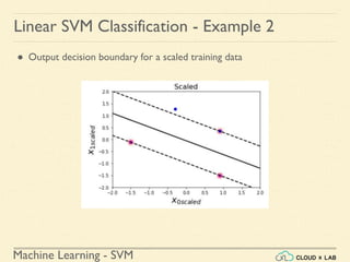
Linear SVM Classification - Example 2
● Building the model, plotting the decision boundary and the training points
>>> svm_clf.fit(X_scaled, ys)
>>> plt.plot(X_scaled[:, 0][ys==1], X_scaled[:, 1][ys==1], "bo")
>>> plt.plot(X_scaled[:, 0][ys==0], X_scaled[:, 1][ys==0], "ms")
>>> plot_svc_decision_boundary(svm_clf, -2, 2)
>>> plt.ylabel("$x_{1scaled}$", fontsize=20)
>>> plt.xlabel("$x_{0scaled}$", fontsize=20)
>>> plt.title("Scaled", fontsize=16)
>>> plt.axis([-2, 2, -2, 2])](https://image.slidesharecdn.com/5-180514114313/85/Support-Vector-Machines-59-320.jpg)


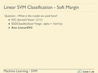
![Machine Learning - SVM
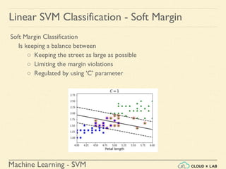
Linear SVM Classification - Soft Margin
Example 1: SVM Classification for IRIS data using c = 1
Steps:
● Load the IRIS data
>>> from sklearn import datasets
>>> from sklearn.pipeline import Pipeline
>>> from sklearn.preprocessing import StandardScaler
>>> from sklearn.svm import LinearSVC
>>> iris = datasets.load_iris()
>>> X = iris["data"][:, (2, 3)] # petal length, petal width
>>> y = (iris["target"] == 2).astype(np.float64) # Iris-Virginica](https://image.slidesharecdn.com/5-180514114313/85/Support-Vector-Machines-77-320.jpg)
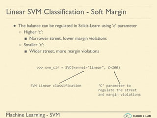
![Machine Learning - SVM
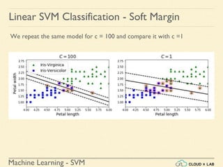
Linear SVM Classification - Soft Margin
Example 1: SVM Classification for IRIS data using c = 1
Steps:
● Load the IRIS data
● Feature scaling the data
● Model the SVM Linear classifier with the training set: fitting
● Test using a sample data
>>> scaled_svm_clf1.predict([[5.5, 1.7]])
array([ 1.])](https://image.slidesharecdn.com/5-180514114313/85/Support-Vector-Machines-79-320.jpg)
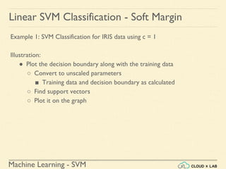
![Machine Learning - SVM
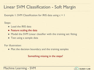
Linear SVM Classification - Soft Margin
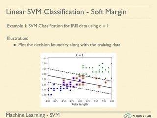
Example 1: SVM Classification for IRIS data using c = 1
Illustration:
● Plot the decision boundary along with the training data
○ Convert to unscaled parameters
# Convert to unscaled parameters
>>> b2 = svm_clf1.decision_function([-scaler.mean_ / scaler.scale_])
>>> w2 = svm_clf1.coef_[0] / scaler.scale_
>>> svm_clf1.intercept_ = np.array([b2])
>>> svm_clf1.coef_ = np.array([w2])](https://image.slidesharecdn.com/5-180514114313/85/Support-Vector-Machines-81-320.jpg)
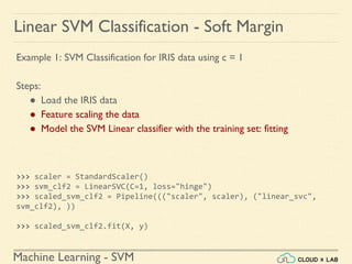
![Machine Learning - SVM
Linear SVM Classification - Soft Margin
Example 1: SVM Classification for IRIS data using c = 1
Illustration:
● Plot the decision boundary along with the training data
○ Find support vectors
# Find support vectors (LinearSVC does not do this automatically)
>>> t = y * 2 - 1
>>> support_vectors_idx2 = (t * (X.dot(w2) + b2) < 1).ravel()
>>> svm_clf1.support_vectors_ = X[support_vectors_idx2]](https://image.slidesharecdn.com/5-180514114313/85/Support-Vector-Machines-82-320.jpg)
![Machine Learning - SVM
Linear SVM Classification - Soft Margin
Example 1: SVM Classification for IRIS data using c = 1
Illustration:
● Plot the decision boundary along with the training data
○ Plot
>>> plt.plot(X[:, 0][y==1], X[:, 1][y==1], "g^")
>>> plt.plot(X[:, 0][y==0], X[:, 1][y==0], "bs")
>>> plot_svc_decision_boundary(svm_clf2, 4, 6)
>>> plt.xlabel("Petal length", fontsize=14)
>>> plt.title("$C = {}$".format(svm_clf2.C), fontsize=16)
>>> plt.axis([4, 6, 0.8, 2.8])
>>> plt.show()](https://image.slidesharecdn.com/5-180514114313/85/Support-Vector-Machines-83-320.jpg)


![Machine Learning - SVM
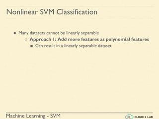
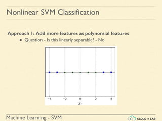
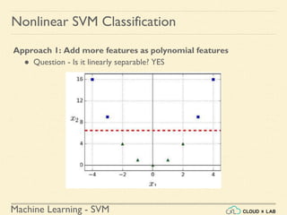
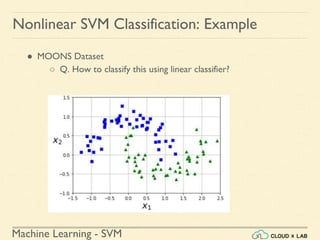
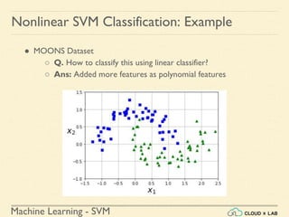
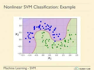
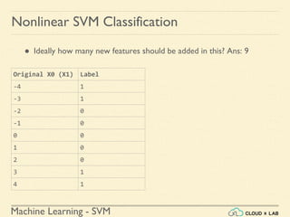
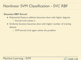
Nonlinear SVM Classification: Example
● MOONS Dataset
>>> from sklearn.datasets import make_moons
>>> X, y = make_moons(n_samples=5, noise=0.15, random_state=42)
Result:
[[-0.92892087 0.20526752]
[ 1.86247597 0.48137792]
[-0.30164443 0.42607949]
[ 1.05888696 -0.1393777 ]
[ 1.01197477 -0.52392748]]
[0 1 1 0 1]
No. of samples
seed](https://image.slidesharecdn.com/5-180514114313/85/Support-Vector-Machines-99-320.jpg)
![Machine Learning - SVM
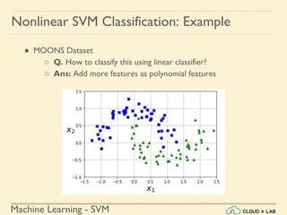
Nonlinear SVM Classification: Example
● MOONS Dataset
Result:
[[-0.92892087 0.20526752]
[ 1.86247597 0.48137792]
[-0.30164443 0.42607949]
[ 1.05888696 -0.1393777 ]
[ 1.01197477 -0.52392748]]
[0 1 1 0 1]](https://image.slidesharecdn.com/5-180514114313/85/Support-Vector-Machines-100-320.jpg)
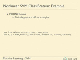
![Machine Learning - SVM
Nonlinear SVM Classification: Example
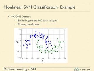
● MOONS Dataset
○ Similarly generate 100 such samples
○ Plotting the dataset
>>> def plot_dataset(X, y, axes):
>>> plt.plot(X[:, 0][y==0], X[:, 1][y==0], "bs")
>>> plt.plot(X[:, 0][y==1], X[:, 1][y==1], "g^")
>>> plt.axis(axes)
>>> plt.grid(True, which='both')
>>> plt.xlabel(r"$x_1$", fontsize=20)
>>> plt.ylabel(r"$x_2$", fontsize=20, rotation=0)
>>> plot_dataset(X, y, [-1.5, 2.5, -1, 1.5])
>>> plt.show()](https://image.slidesharecdn.com/5-180514114313/85/Support-Vector-Machines-102-320.jpg)
![Machine Learning - SVM
Nonlinear SVM Classification: Example
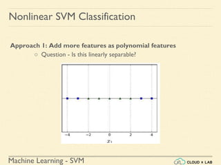
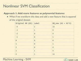
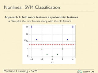
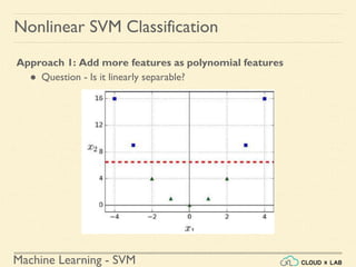
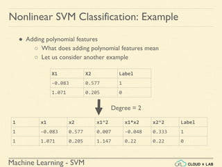
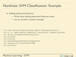
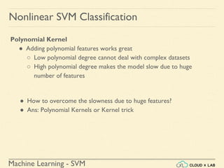
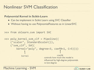
● Adding polynomial features
○ What does adding polynomial features mean
○ Let us consider another example
X = [[-0.08 0.58]
[ 1.07 0.21]]
y = [1 0]
X1 =
[[ 1. -0.08 0.58 0.01 -0.05 0.33 -0. 0. -0.03 0.19]
[ 1. 1.07 0.21 1.15 0.22 0.04 1.23 0.24 0.05 0.01]]](https://image.slidesharecdn.com/5-180514114313/85/Support-Vector-Machines-108-320.jpg)
![Machine Learning - SVM
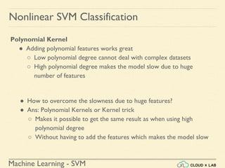
Nonlinear SVM Classification: Example
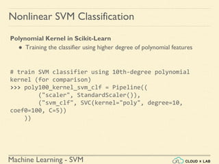
def plot_predictions(clf, axes):
x0s = np.linspace(axes[0], axes[1], 100)
x1s = np.linspace(axes[2], axes[3], 100)
x0, x1 = np.meshgrid(x0s, x1s)
X = np.c_[x0.ravel(), x1.ravel()]
y_pred = clf.predict(X).reshape(x0.shape)
y_decision = clf.decision_function(X).reshape(x0.shape)
plt.contourf(x0, x1, y_pred, cmap=plt.cm.brg, alpha=0.2)
plt.contourf(x0, x1, y_decision, cmap=plt.cm.brg, alpha=0.1)
plot_predictions(polynomial_svm_clf, [-1.5, 2.5, -1, 1.5])
plot_dataset(X, y, [-1.5, 2.5, -1, 1.5])
plt.show()](https://image.slidesharecdn.com/5-180514114313/85/Support-Vector-Machines-113-320.jpg)


![Machine Learning - SVM
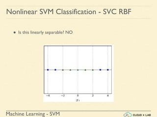
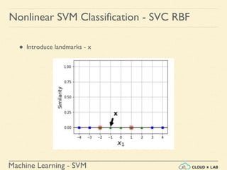
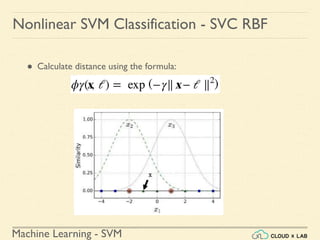
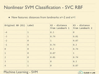
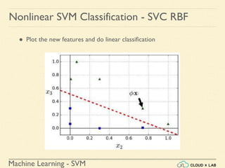
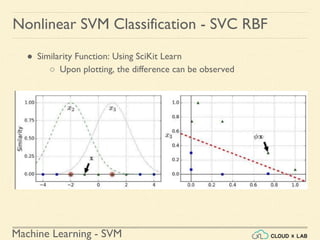
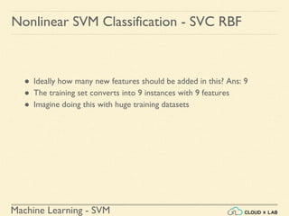
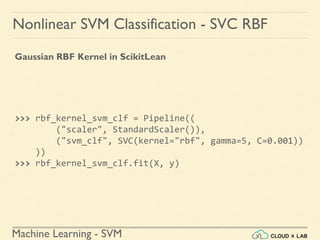
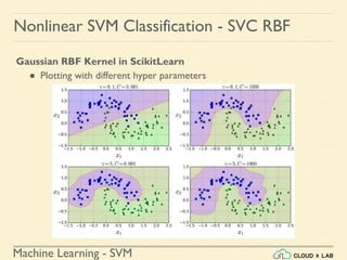
Nonlinear SVM Classification - SVC RBF
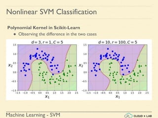
● Similarity Function: Using SciKit Learn
# define similarity function to be Gaussian Radial Basis Function
(RBF)
# equals 0 (far away) to 1 (at landmark)
>>> def gaussian_rbf(x, landmark, gamma):
return np.exp(-gamma * np.linalg.norm(x - landmark, axis=1)**2)
>>> gamma = 0.3
>>> x1s = np.linspace(-4.5, 4.5, 200).reshape(-1, 1)
>>> x2s = gaussian_rbf(x1s, -2, gamma)
>>> x3s = gaussian_rbf(x1s, 1, gamma)
>>> XK = np.c_[gaussian_rbf(X1D, -2, gamma), gaussian_rbf(X1D, 1,
gamma)]
>>> yk = np.array([0, 0, 1, 1, 1, 1, 1, 0, 0])
>>> print(XK)](https://image.slidesharecdn.com/5-180514114313/85/Support-Vector-Machines-130-320.jpg)


![Machine Learning - SVM
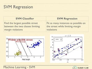
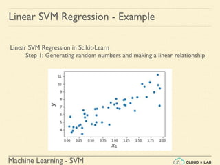
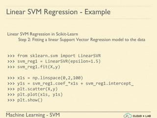
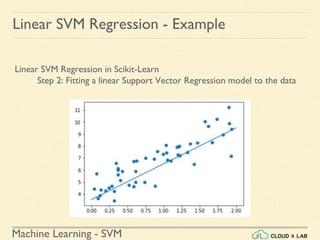
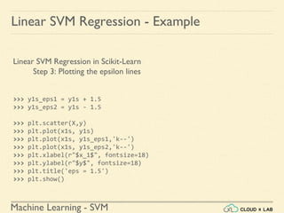
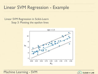
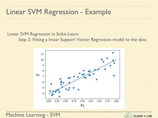
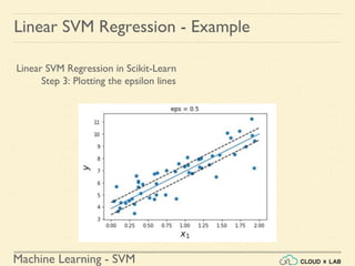
Linear SVM Regression - Example
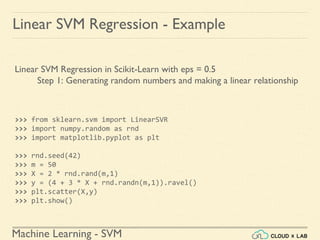
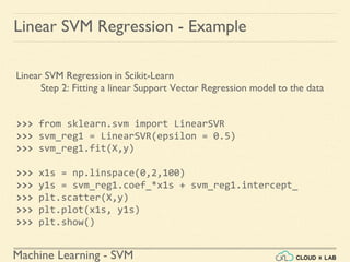
Linear SVM Regression in Scikit-Learn
Step 4: Finding the instances off-the-street and plotting
>>> y_pred = svm_reg1.predict(X)
>>> supp_vec_X = X[np.abs(y-y_pred)>1.5]
>>> supp_vec_y = y[np.abs(y-y_pred)>1.5]
>>> plt.scatter(supp_vec_X,supp_vec_y)
>>> plt.show()](https://image.slidesharecdn.com/5-180514114313/85/Support-Vector-Machines-158-320.jpg)


![Machine Learning - SVM
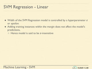
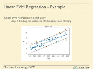
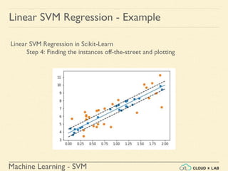
Linear SVM Regression - Example
Linear SVM Regression in Scikit-Learn
Step 4: Finding the instances off-the-street and plotting
>>> y_pred = svm_reg1.predict(X)
>>> supp_vec_X = X[np.abs(y-y_pred)>0.5]
>>> supp_vec_y = y[np.abs(y-y_pred)>0.5]
>>> plt.scatter(supp_vec_X,supp_vec_y)
>>> plt.show()](https://image.slidesharecdn.com/5-180514114313/85/Support-Vector-Machines-167-320.jpg)


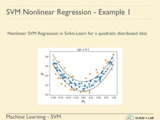
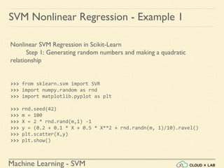
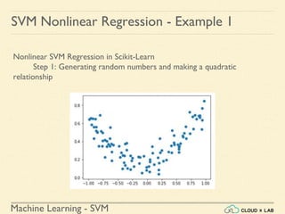
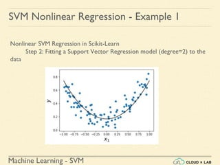
![Machine Learning - SVM
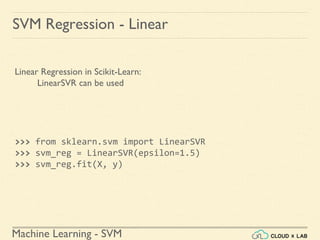
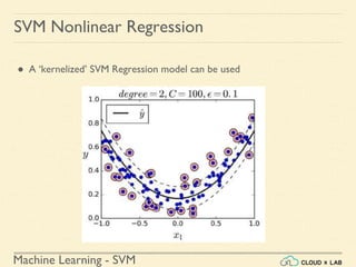
Nonlinear SVM Regression in Scikit-Learn
Step 2: Fitting a Support Vector Regression model (degree=2) to the
data
>>> from sklearn.svm import SVR
>>> svr_poly_reg1 = SVR(kernel="poly", degree=2, C =
100, epsilon = 0.1)
>>> svr_poly_reg1.fit(X,y)
>>> print(svr_poly_reg1.C)
>>> x1s = np.linspace(-1,1,200)
>>> plot_svm_regression(svr_poly_reg1, X, y, [-1, 1, 0,
1])
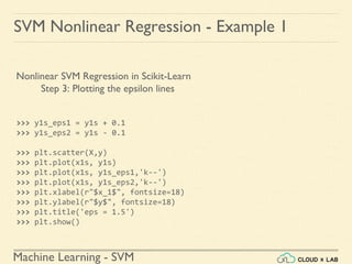
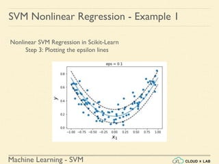
SVM Nonlinear Regression - Example 1](https://image.slidesharecdn.com/5-180514114313/85/Support-Vector-Machines-179-320.jpg)
![Machine Learning - SVM
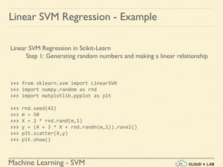
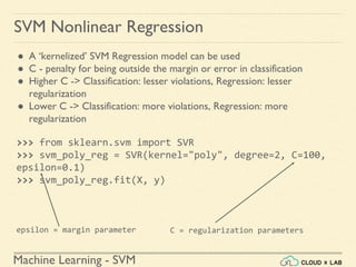
Nonlinear SVM Regression in Scikit-Learn
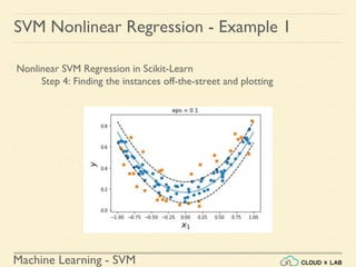
Step 4: Finding the instances off-the-street and plotting
>>> y1_predict = svr_poly_reg1.predict(X)
>>> supp_vectors_X = X[np.abs(y-y1_predict)>0.1]
>>> supp_vectors_y = y[np.abs(y-y1_predict)>0.1]
>>> plt.scatter(supp_vectors_X ,supp_vectors_y)
>>> plt.show()
SVM Nonlinear Regression - Example 1](https://image.slidesharecdn.com/5-180514114313/85/Support-Vector-Machines-183-320.jpg)


![Machine Learning - SVM
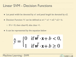
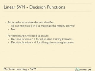
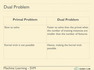
Linear SVM - Decision Functions
What do we know?
- For a 2d dataset, the slope of the margin is equal to w = [w1, w2] and
the slope of the decision boundary is equal to w1^2 + w2^2
- For a n-dimensional dataset, w = [w1, w2, w3, ... , wn] and the slope of
the decision function is denoted by || w ||](https://image.slidesharecdn.com/5-180514114313/85/Support-Vector-Machines-198-320.jpg)


The document discusses Support Vector Machines (SVM) in machine learning, emphasizing their capabilities for linear and nonlinear classification, regression, and outlier detection, particularly suited for small to medium datasets. It outlines the process of training and testing SVM models, the importance of feature scaling, and differences between hard and soft margin classifications. Examples include various classification types, such as binary, multi-class, and multi-label, illustrated using datasets like the Iris dataset.


![SVM[Support vector Machine] Machine learning](https://cdn.slidesharecdn.com/ss_thumbnails/svm-250403184638-1cd9afdb-thumbnail.jpg?width=640&height=640&fit=bounds)