The document provides an overview of various clustering strategies, machine learning frameworks, and classifier types, emphasizing the importance of model generalization and the impact of training size on prediction accuracy. It discusses different classification methods such as nearest neighbor, linear classifiers, and support vector machines, while also addressing the bias-variance tradeoff and the need for appropriate feature representation. Additionally, it touches on the process of selecting kernels for image classification with SVMs and highlights the pros and cons of different classifiers.

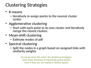
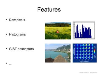
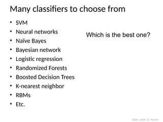
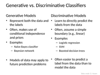
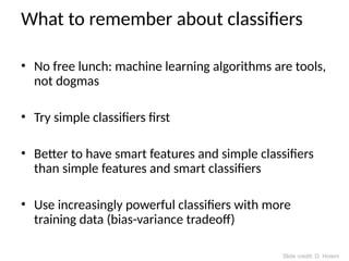
2. Clustering Strategies
• K-means
– Iteratively re-assign points to the nearest cluster
center
• Agglomerative clustering
– Start with each point as its own cluster and iteratively
merge the closest clusters
• Mean-shift clustering
– Estimate modes of pdf
• Spectral clustering
– Split the nodes in a graph based on assigned links with
similarity weights
As we go down this chart, the clustering strategies
have more tendency to transitively group points
even if they are not nearby in feature space

4. The machine learning
framework
• Apply a prediction function to a feature representation of the
image to get the desired output:
f( ) = “apple”
f( ) = “tomato”
f( ) = “cow”
Slide credit: L. Lazebnik

5. The machine learning
framework
y = f(x)
• Training: given a training set of labeled examples {(x1,y1), …,
(xN,yN)}, estimate the prediction function f by minimizing the
prediction error on the training set
• Testing: apply f to a never before seen test example x and output
the predicted value y = f(x)
output prediction
function
Image
feature
Slide credit: L. Lazebnik

6. Prediction
Steps
Training
Labels
Training
Images
Training
Training
Image
Features
Image
Features
Testing
Test Image
Learned
model
Learned
model
Slide credit: D. Hoiem and L. Lazebnik

7. Features
• Raw pixels
• Histograms
• GIST descriptors
• …
Slide credit: L. Lazebnik

8. Classifiers: Nearest neighbor
f(x) = label of the training example nearest to x
• All we need is a distance function for our inputs
• No training required!
Test
example
Training
examples
from class 1
Training
examples
from class 2
Slide credit: L. Lazebnik

9. Classifiers: Linear
• Find a linear function to separate the classes:
f(x) = sgn(w  x + b)
Slide credit: L. Lazebnik

10. Many classifiers to choose from
• SVM
• Neural networks
• Naïve Bayes
• Bayesian network
• Logistic regression
• Randomized Forests
• Boosted Decision Trees
• K-nearest neighbor
• RBMs
• Etc.
Which is the best one?
Slide credit: D. Hoiem

11. • Images in the training set must be annotated with the
“correct answer” that the model is expected to produce
Contains a motorbike
Recognition task and supervision
Slide credit: L. Lazebnik

12. Unsupervised “Weakly” supervised Fully supervised
Definition depends on task
Slide credit: L. Lazebnik

13. Generalization
• How well does a learned model generalize from the
data it was trained on to a new test set?
Training set (labels known) Test set (labels
unknown)
Slide credit: L. Lazebnik

14. Generalization
• Components of generalization error
– Bias: how much the average model over all training sets differ from
the true model?
• Error due to inaccurate assumptions/simplifications made by the
model
– Variance: how much models estimated from different training sets
differ from each other
• Underfitting: model is too “simple” to represent all the
relevant class characteristics
– High bias and low variance
– High training error and high test error
• Overfitting: model is too “complex” and fits irrelevant
characteristics (noise) in the data
– Low bias and high variance
– Low training error and high test error
Slide credit: L. Lazebnik

15. Effect of Training Size
Testing
Training
Generalization Error
Number of Training Examples
Error
Fixed prediction model
Slide credit: D. Hoiem

16. Remember…
• No classifier is inherently
better than any other: you
need to make assumptions to
generalize
• Three kinds of error
– Inherent: unavoidable
– Bias: due to over-simplifications
– Variance: due to inability to
perfectly estimate parameters
from limited data
Slide credit: D. Hoiem
Slide credit: D. Hoiem

17. How to reduce variance?
• Choose a simpler classifier
• Regularize the parameters
• Get more training data
Slide credit: D. Hoiem

18. Very brief tour of some classifiers
• K-nearest neighbor
• SVM
• Boosted Decision Trees
• Neural networks
• Naïve Bayes
• Bayesian network
• Logistic regression
• Randomized Forests
• RBMs
• Etc.

19. Generative vs. Discriminative Classifiers
Generative Models
• Represent both the data and
the labels
• Often, makes use of
conditional independence
and priors
• Examples
– Naïve Bayes classifier
– Bayesian network
• Models of data may apply to
future prediction problems
Discriminative Models
• Learn to directly predict the
labels from the data
• Often, assume a simple
boundary (e.g., linear)
• Examples
– Logistic regression
– SVM
– Boosted decision trees
• Often easier to predict a
label from the data than to
model the data
Slide credit: D. Hoiem

20. Classification
• Assign input vector to one of two or more
classes
• Any decision rule divides input space into
decision regions separated by decision
boundaries
Slide credit: L. Lazebnik

21. Nearest Neighbor Classifier
• Assign label of nearest training data point to each test data
point
Voronoi partitioning of feature space
for two-category 2D and 3D data
from Duda et al.
Source: D. Lowe

22. K-nearest neighbor
x x
x
x
x
x
x
x
o
o
o
o
o
o
o
x2
x1
+
+

23. 1-nearest neighbor
x x
x
x
x
x
x
x
o
o
o
o
o
o
o
x2
x1
+
+

24. 3-nearest neighbor
x x
x
x
x
x
x
x
o
o
o
o
o
o
o
x2
x1
+
+

25. 5-nearest neighbor
x x
x
x
x
x
x
x
o
o
o
o
o
o
o
x2
x1
+
+

26. Using K-NN
• Simple, a good one to try first
• With infinite examples, 1-NN provably has
error that is at most twice Bayes optimal error

27. Classifiers: Linear SVM
x x
x
x
x
x
x
x
o
o
o
o
o
x2
x1
• Find a linear function to separate the classes:
f(x) = sgn(w  x + b)

28. Classifiers: Linear SVM
x x
x
x
x
x
x
x
o
o
o
o
o
x2
x1
• Find a linear function to separate the classes:
f(x) = sgn(w  x + b)

29. Classifiers: Linear SVM
x x
x
x
x
x
x
x
o
o
o
o
o
o
x2
x1
• Find a linear function to separate the classes:
f(x) = sgn(w  x + b)

30. • Datasets that are linearly separable work out great:
• But what if the dataset is just too hard?
• We can map it to a higher-dimensional space:
0 x
0 x
0 x
x2
Nonlinear SVMs
Slide credit: Andrew Moore

31. Φ: x → φ(x)
Nonlinear SVMs
• General idea: the original input space can
always be mapped to some higher-dimensional
feature space where the training set is
separable:
Slide credit: Andrew Moore

32. Nonlinear SVMs
• The kernel trick: instead of explicitly computing
the lifting transformation φ(x), define a kernel
function K such that
K(xi,xj) = φ(xi )· φ(xj)
(to be valid, the kernel function must satisfy
Mercer’s condition)
• This gives a nonlinear decision boundary in the
original feature space:
b
K
y
b
y
i
i
i
i
i
i
i
i 


 
 )
,
(
)
(
)
( x
x
x
x 



C. Burges, A Tutorial on Support Vector Machines for Pattern Recognition, Data Mining
and Knowledge Discovery, 1998

33. Nonlinear kernel: Example
• Consider the mapping )
,
(
)
( 2
x
x
x 

2
2
2
2
2
2
)
,
(
)
,
(
)
,
(
)
(
)
(
y
x
xy
y
x
K
y
x
xy
y
y
x
x
y
x









x2

34. Kernels for bags of features
• Histogram intersection kernel:
• Generalized Gaussian kernel:
• D can be (inverse) L1 distance, Euclidean
distance, χ2
distance, etc.



N
i
i
h
i
h
h
h
I
1
2
1
2
1 ))
(
),
(
min(
)
,
(







 2
2
1
2
1 )
,
(
1
exp
)
,
( h
h
D
A
h
h
K
J. Zhang, M. Marszalek, S. Lazebnik, and C. Schmid,
Local Features and Kernels for Classifcation of Texture and Object Categories: A Compr
ehensive Study

35. Summary: SVMs for image classification
1. Pick an image representation (in our case, bag
of features)
2. Pick a kernel function for that representation
3. Compute the matrix of kernel values between
every pair of training examples
4. Feed the kernel matrix into your favorite SVM
solver to obtain support vectors and weights
5. At test time: compute kernel values for your test
example and each support vector, and combine
them with the learned weights to get the value of
the decision function
Slide credit: L. Lazebnik

36. What about multi-class SVMs?
• Unfortunately, there is no “definitive” multi-
class SVM formulation
• In practice, we have to obtain a multi-class
SVM by combining multiple two-class SVMs
• One vs. others
• Traning: learn an SVM for each class vs. the others
• Testing: apply each SVM to test example and assign to it the
class of the SVM that returns the highest decision value
• One vs. one
• Training: learn an SVM for each pair of classes
• Testing: each learned SVM “votes” for a class to assign to
the test example
Slide credit: L. Lazebnik

37. SVMs: Pros and cons
• Pros
• Many publicly available SVM packages:
http://www.kernel-machines.org/software
• Kernel-based framework is very powerful, flexible
• SVMs work very well in practice, even with very small
training sample sizes
• Cons
• No “direct” multi-class SVM, must combine two-class SVMs
• Computation, memory
– During training time, must compute matrix of kernel values for
every pair of examples
– Learning can take a very long time for large-scale problems

38. What to remember about classifiers
• No free lunch: machine learning algorithms are tools,
not dogmas
• Try simple classifiers first
• Better to have smart features and simple classifiers
than simple features and smart classifiers
• Use increasingly powerful classifiers with more
training data (bias-variance tradeoff)
Slide credit: D. Hoiem

39. Some Machine Learning References
• General
– Tom Mitchell, Machine Learning, McGraw Hill, 1997
– Christopher Bishop, Neural Networks for Pattern
Recognition, Oxford University Press, 1995
• Adaboost
– Friedman, Hastie, and Tibshirani, “Additive logistic
regression: a statistical view of boosting”, Annals of
Statistics, 2000
• SVMs
– http://www.support-vector.net/icml-tutorial.pdf
Slide credit: D. Hoiem