Downloaded 785 times
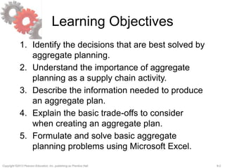
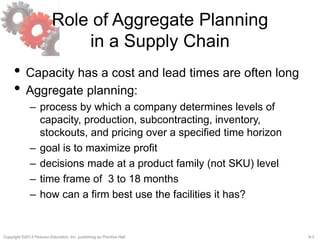
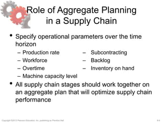
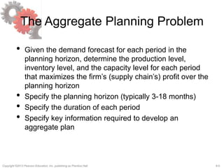
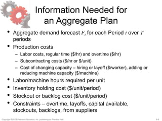
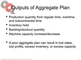
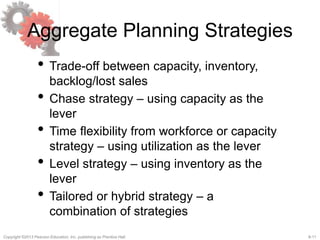
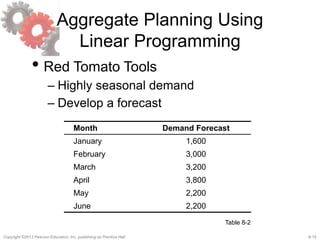
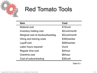
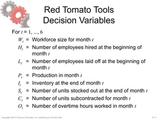
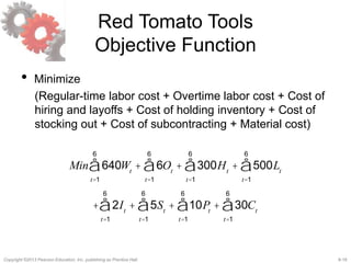
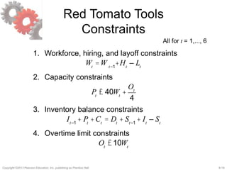
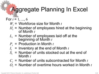
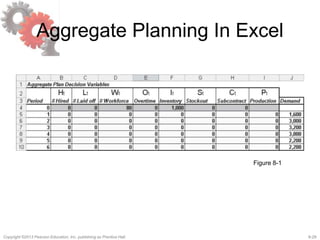
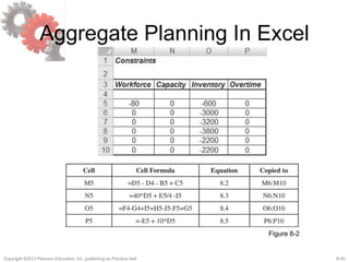
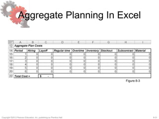

This document discusses aggregate planning and its role in supply chain management. It begins by defining aggregate planning as the process of determining optimal levels of production, capacity, inventory, and other factors over a 3-18 month time horizon. The document then provides learning objectives, outlines key information needed for aggregate planning like demand forecasts and cost data, and describes different aggregate planning strategies like chase, level, and time flexibility strategies. It concludes by presenting an example aggregate planning problem for a company called Red Tomato Tools using linear programming.