Downloaded 670 times

![7-10Copyright ©2013 Pearson Education, Inc. publishing as Prentice Hall.
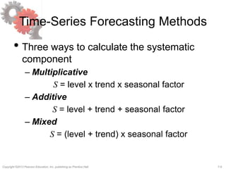
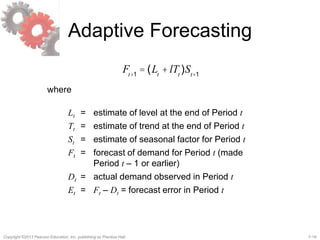
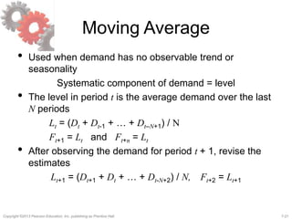
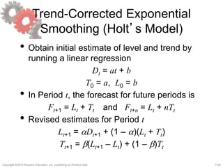
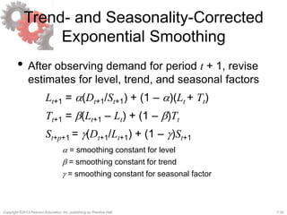
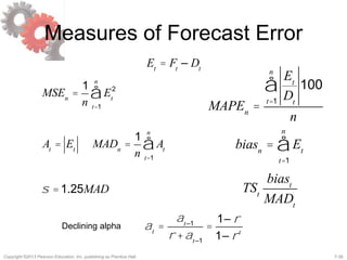
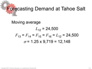
Static Methods
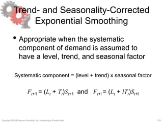
Systematic component = (level+ trend)´seasonal factor
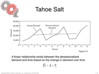
Ft+l
= [L+(t + l)T]St+l
where
L = estimate of level at t = 0
T = estimate of trend
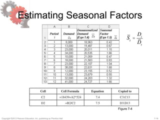
St = estimate of seasonal factor for Period t
Dt = actual demand observed in Period t
Ft = forecast of demand for Period t](https://image.slidesharecdn.com/choprascm5ch07-150901035624-lva1-app6892/85/Supply-Chain-Management-chap-7-10-320.jpg)
![7-13Copyright ©2013 Pearson Education, Inc. publishing as Prentice Hall.
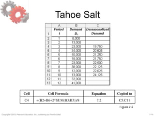
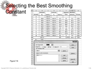
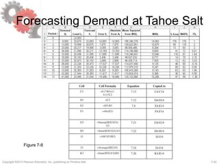
Estimate Level and Trend
Periodicity p = 4, t = 3
Dt
=
Dt–( p/2)
+ Dt+( p/2)
+ 2Di
i=t+1–( p/2)
t–1+( p/2)
å
é
ë
ê
ê
ù
û
ú
ú
/ (2p) for p even
Di
/ p for p odd
i=t–[( p–1)/2]
t+[( p–1)/2]
å
ì
í
ï
ï
î
ï
ï
Dt
= Dt–( p/2)
+ Dt+( p/2)
+ 2Di
i=t+1–( p/2)
t–1+( p/2)
å
é
ë
ê
ê
ù
û
ú
ú
/ (2p)
= D1
+ D5
+ 2Di
i=2
4
å / 8](https://image.slidesharecdn.com/choprascm5ch07-150901035624-lva1-app6892/85/Supply-Chain-Management-chap-7-13-320.jpg)

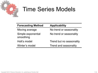

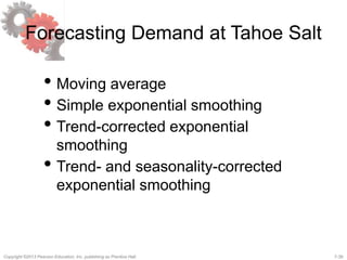
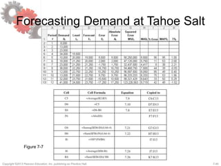


This document discusses demand forecasting in supply chains. It covers the role of forecasting, characteristics of forecasts, components of forecasts, and time-series forecasting methods. The key methods covered are static, adaptive, moving average, simple exponential smoothing, Holt's exponential smoothing (for trend), and Winter's method (for trend and seasonality). Examples are provided to illustrate how to apply these forecasting techniques to real demand data. The overall goal of the techniques is to decompose historical demand data into systematic and random components to generate accurate forecasts.