The document explains measures of central tendency, specifically mean, median, and mode, as ways to describe a set of data with a single representative value. It outlines how to compute these measures for both ungrouped and grouped data, including examples and formulas. Additionally, it discusses the pros and cons of each measure, illustrating their applicability and limitations.

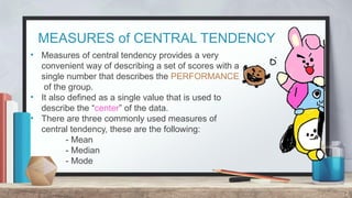
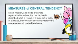
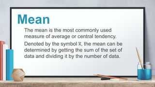
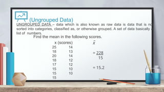
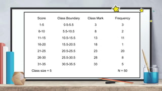
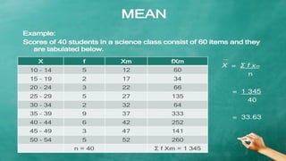
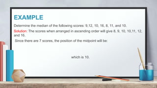
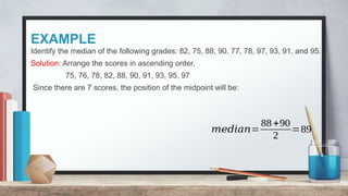
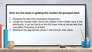
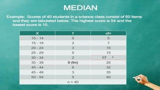
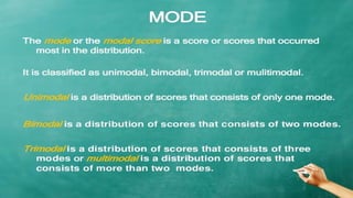
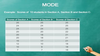
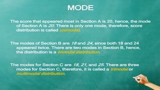
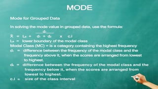
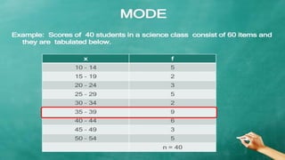
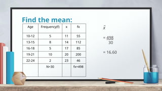
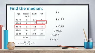
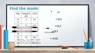
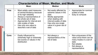
1. Measures
of
Central Tendency:

2. MEASURES of CENTRAL TENDENCY
2
• Measures of central tendency provides a very
convenient way of describing a set of scores with a
single number that describes the PERFORMANCE
of the group.
• It also defined as a single value that is used to
describe the “center” of the data.
• There are three commonly used measures of
central tendency, these are the following:
- Mean
- Median
- Mode

3. MEASURES of CENTRAL TENDENCY
3
Mean, median, and mode are single
representative values that can be used to
described what is typical in a large set of data.
In statistics, these values collectively referred to
as measures of central tendency.

4. Mean
The mean is the most commonly used
measure of average or central tendency.
Denoted by the symbol , the mean can be
x
̅
determined by getting the sum of the set of
data and dividing it by the number of data.
4

5. 5
Computation of mean for:
Ungrouped data Grouped data
x̅ x̅

6. (Ungrouped Data)
Find the mean in the following scores.
6
x (scores)
25 14
18 13
20 14
18 12
17 12
15 10
15 10
15
x
̅
= 228
15
= 15.2
UNGROUPED DATA – data which is also known as raw data is data that is not
sorted into categories, classified as, or otherwise grouped. A set of data basically a
list of numbers.

7. where gives the individual scores and the corresponding weights of each
score.
7
Example: Find the grade point average of Jen if she obtained the grades of 87,
90, 82, and 80 each having 2, 1.8, 1.5, and 1.2 units respectively.
Sometimes each individual score has different levels of significance, or weights,
and you are asked to get the mean. In this case, you have to specifically obtain
the weighted mean, which can be determined by dividing the sum of the products
and the weights by the total weights. Thus,
𝑤𝑒𝑖𝑔 h𝑡𝑒𝑑𝑚𝑒𝑎𝑛=
87 (2)+90 (1 .8)+82(1.5)+80 (1.2)
6.5
𝑤𝑒𝑖𝑔 h𝑡𝑒𝑑𝑚𝑒𝑎𝑛=
174 +162+123+96
6 .5
𝑤𝑒𝑖𝑔 h𝑡𝑒𝑑𝑚𝑒𝑎𝑛=
174 +162+123+96
6 .5
𝒘𝒆𝒊𝒈𝒉𝒕𝒆𝒅 𝒎𝒆𝒂𝒏=
555
6.5
≈85 .38

8. “
MEAN for GROUPED DATA
8
Grouped Data are the data or scores that are
arranged in a frequency distribution.
Frequency Distribution is the arrangement of scores
according to category of classes including the
frequency.

9. TERMINOLOGIES (Recall)
Class Interval
Class Limits
Class Size(Class Width)
Frequency
Class Boundaries
Classmark (Midpoint)

10. CLASS INTERVAL
Class intervals or classes, are the groups of values that
function as row classifiers. In the above example, the class
intervals are 1-5, 6-10, 11-15, 16-20, etc.

11. CLASS LIMITS
Class limits are the smallest and largest possible values that
can fall into each class interval. The smaller number in the
class interval is called the lower limit, whereas the larger
number is the upper limit. The numbers 1, 6, 11, …31 are
lower limits, and the numbers 5, 10, 15, 20, … 35 are upper
limits.

12. CLASS SIZE or CLASS WIDTH
Class size or class width is the number of values that are
contained in each class. The size is uniform to all classes of
the frequency distribution table. Class size can be determined
by subtracting two successive lower limits or two consecutive
upper limits. In the previous sample frequency distribution
table, the class size is 5 since the difference between two
consecutive lower limits or upper limits is 5 (i.e., 6-1=5 or10-
5=5).

13. FREQUENCY
Frequency is the number of cases falling into each class
interval. The previous table is just an example of simple
frequency distribution. A complete distribution table includes
other parts such as class boundary, class mark, relative
frequency, and cumulative frequency.

14. CLASS BOUNDARIES
Class boundaries, also known as true limits, are obtained by
subtracting 0.5 to the lower limit and adding 0.5 to upper limit
of each class. This is always true when the class limits are
whole numbers. However, note that if data are in one decimal
place, you subtract or add 0.05 to get the class boundaries,
and 0.005 for two-decimal limits. Class boundaries are very
useful when dealing with continuous type of data.

15. CLAClass mark, denoted by , is
the midpoint of a class interval.
This can be obtained by
dividing the sum of the upper
limit (UL) and the lower limit
(LL) of the class interval by 2SS
MARK
Class mark, denoted by , is the midpoint of a class interval.
This can be obtained by dividing the sum of the upper limit
(UL) and the lower limit (LL) of the class interval by 2, thus, .
For example in the first class the class mark will be

16. Score Class Boundary Class Mark Frequency
1-5 0.5-5.5 3 3
6-10 5.5-10.5 8 2
11-15 10.5-15.5 13 11
16-20 15.5-20.5 18 1
21-25 20.5-25.5 23 20
26-30 25.5-30.5 28 8
31-35 30.5-35.5 33 5
Class size = 5 N = 50

17. “
17

18. To simplify the process, follow the steps:
1. Compute the class marks of each class.
2. Multiply each class mark by the corresponding frequencies.
3. Get the summation of all products in step 2.
4. Divide the summation of the products by the total number of
observations.

19. “
19

22. MEDIAN
The median refers to the middle value in a set
of data. It may be obtained by arranging the
scores in either ascending or descending
order and then locating the
22

23. EXAMPLE
Determine the median of the following scores: 9,12, 10, 16, 8, 11, and 10.
Solution: The scores when arranged in ascending order will give 8, 9, 10, 10,11, 12,
and 16.
Since there are 7 scores, the position of the midpoint will be:
which is 10.
23

24. EXAMPLE
Identify the median of the following grades: 82, 75, 88, 90, 77, 78, 97, 93, 91, and 95.
Solution: Arrange the scores in ascending order.
75, 76, 78, 82, 88, 90, 91, 93, 95, 97
Since there are 7 scores, the position of the midpoint will be:
𝑚𝑒𝑑𝑖𝑎𝑛=
88+90
2
=89

27. Median for Grouped Data
The concepts of class boundary and less than cumulative frequency are
crucial in determining the median for grouped data. To compute for the
mean of grouped data,
use the formula
Where L = lower class boundary of the median class
N= total frequency
F= cumulative frequency before the median class
= frequency of the median class
i = class size/width
Note: The formula above only works when the class interval are arranged in
ascending order.

28. Here are the steps in getting the median for grouped data:
1. Compute the less than cumulative frequencies.
2. Locate the median class. Since the median is the middle value in the
distribution, it can be found on the first class interval whose less than
cumulative frequency is at least .
3. Substitute the appropriate values in the formula, then solve.

31. MODE
The value that appears most frequently in a
given data is called the mode. A distribution
may be classified according to its number of
modes. For example, a set of data is called
unimodal when it has exactly one mode,
bimodal when it contains two modes, and
multimodal when it has many modes. In some
instances, a set of data may have no mode.
31

38. Find the mean:
38
Age Frequency(f) x fx
10-12 5 11 55
13-15 8 14 112
16-18 5 17 85
19-21 10 20 200
22-24 2 23 46
N=30 fx=498
x
̅
= 498
30
= 16.60

39. Find the median:
39
Age Freque
ncy(f)
L.C.B <cf
10-12 5 9.5 5
13-15 8 12.5 13
16-18 5 15.5 18
19-21 10 18.5 28
22-24 2 21.5 30
N=30
x̃ =
x̃ =15.5
x̃ =15.5
x̃ =15.5
x̃ =15.5
x̃ =16.7
x̃ 𝑐=
𝑁
2
=
30
2
=15

40. Find the mode:
40
Age Frequenc
y(f)
L.C.B
10-
12
5 9.5
13-
15
8 12.5
16-
18
5 15.5
19-
21
10 18.5
22-
24
2 21.5
x=
=18.5
=18.5
=18.5
= 19.65
D1 =f𝑚 − f𝑏=10 −5=5
D2=f𝑚 − f𝑎=10− 2=8
D 1
D 2

41. Mean Median Mode
Pros • Most widely used measures
of central tendency because
of its high reliability
• Always a representative of
the whole set of data
• Appropriate for interval and
ratio scales of data
• Has only one value to
describe a set of data
• Not easily affected by
extreme values in the
data
• Mostly appropriate
when dealing with
interval scales of data
• Has only one single
value in a given set of
data.
• Appropriate for nominal
scales of data
• Easy to compute
Cons • Easily influenced by
extremely high or extremely
low scores or values in the
distribution
• Not always a
representative of the
set of data
• Non-uniqueness of the
value since there can be
many modes in a set of
data
• Not reliable
• Not always a
representative
Characteristics of Mean, Median, and Mode

42. Activity
Read and analyze the given problem carefully.
42

43. problem !
1. The table below shows the weights(kg)
of members in a sport club. Calculate the
mean, median and mode of the
distribution.
Masses 40-49 50-59 60-69 70-79 80-89 90-99
Frequency 6 8 12 14 7 3