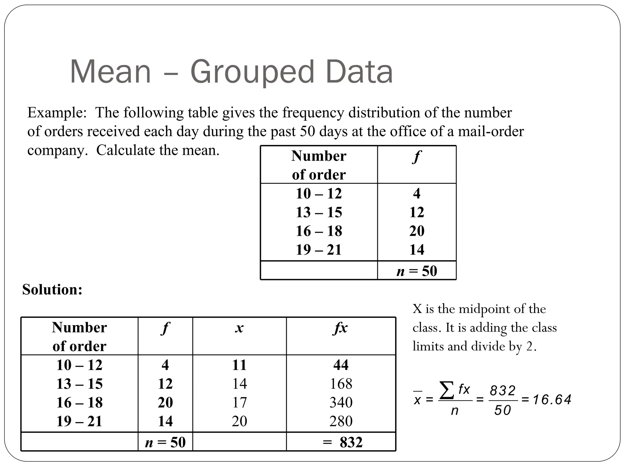
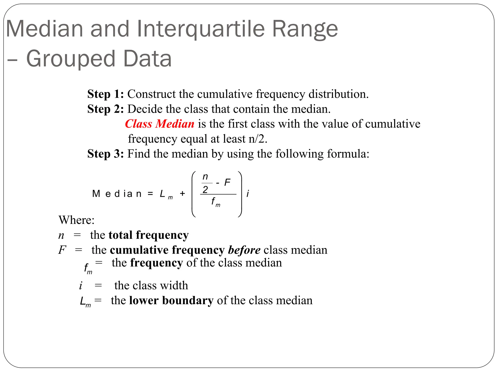
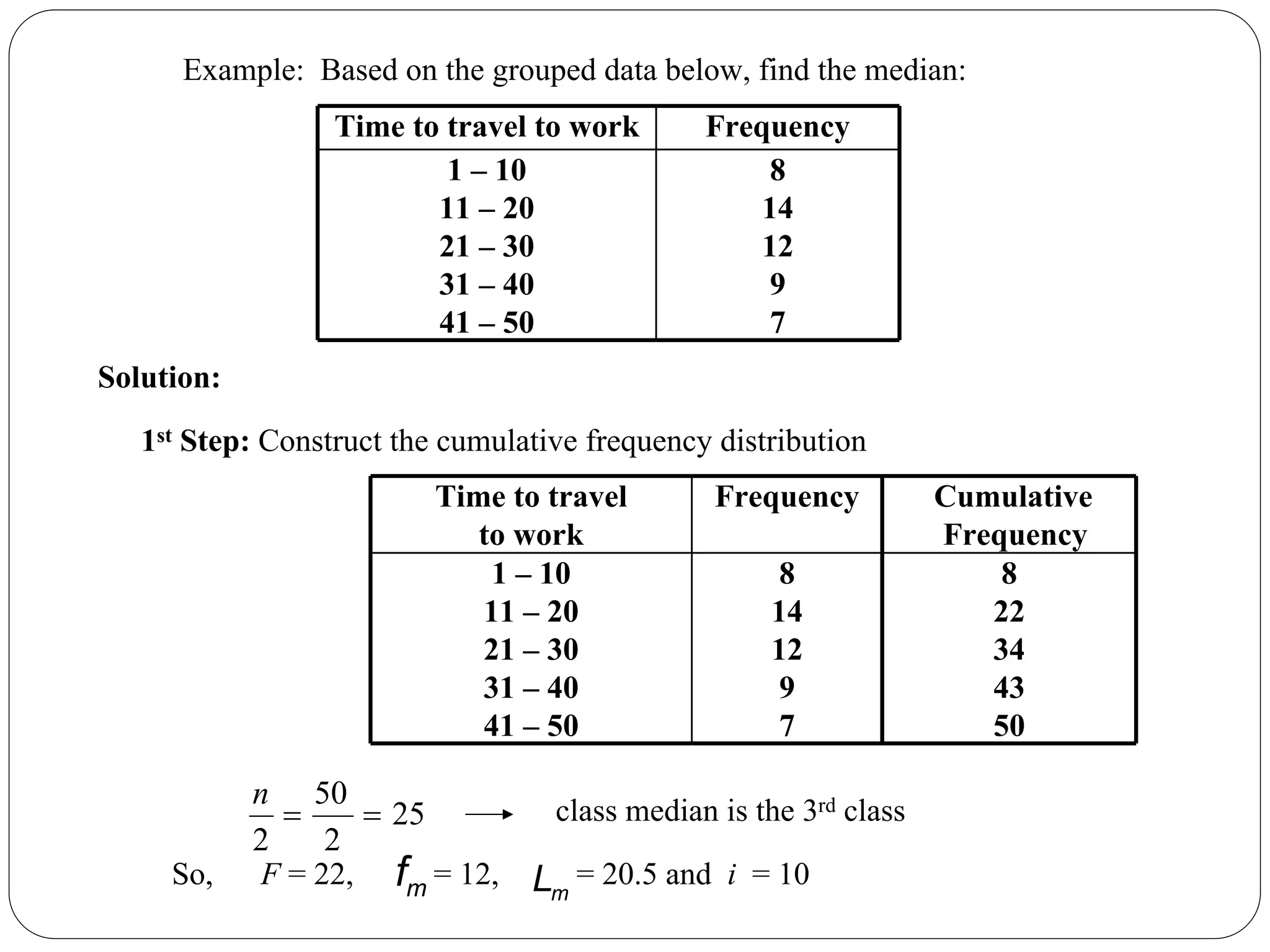
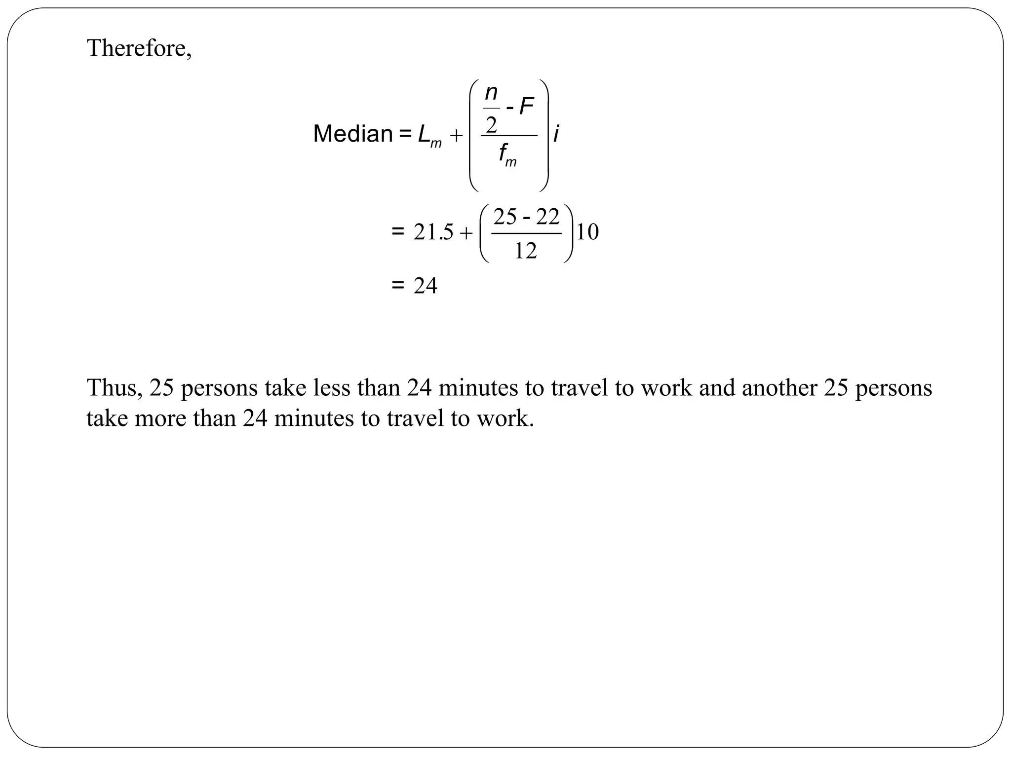
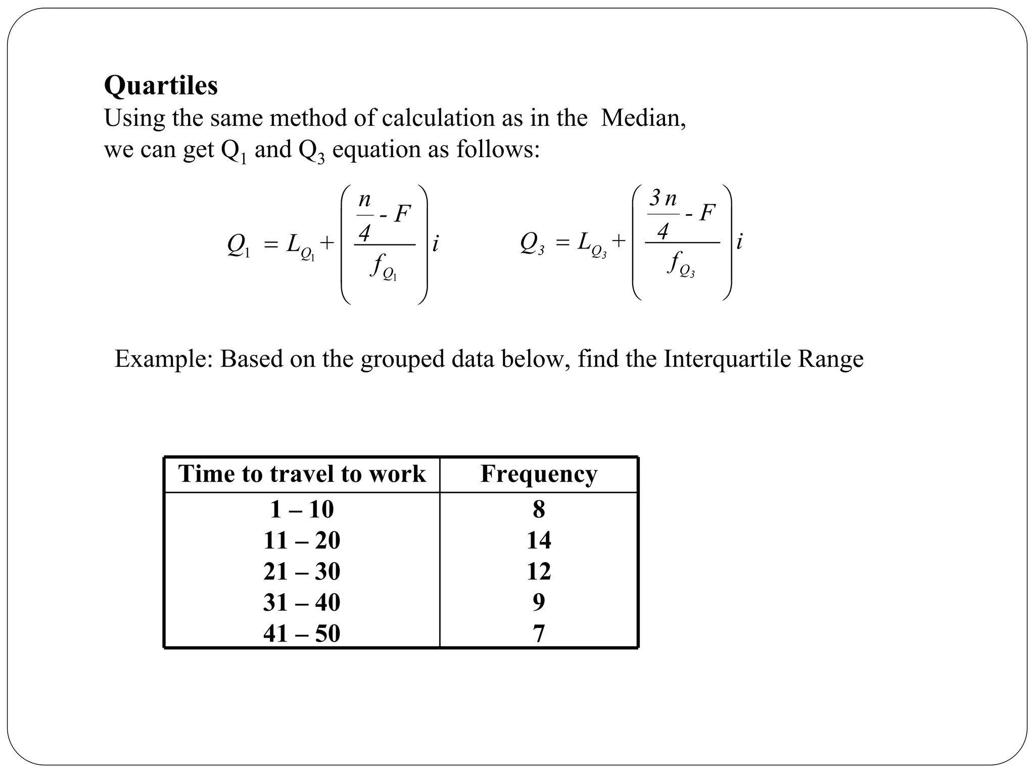
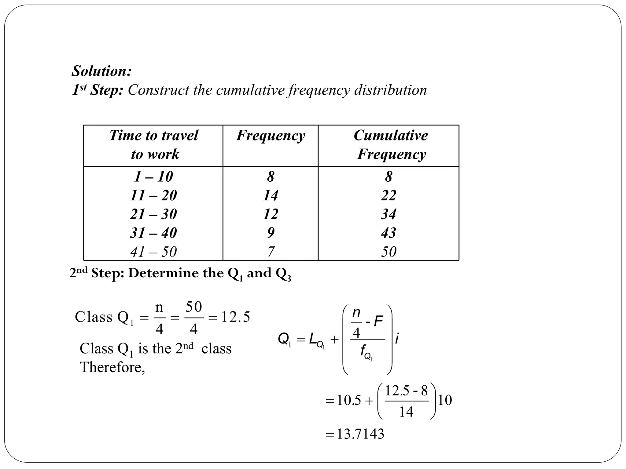
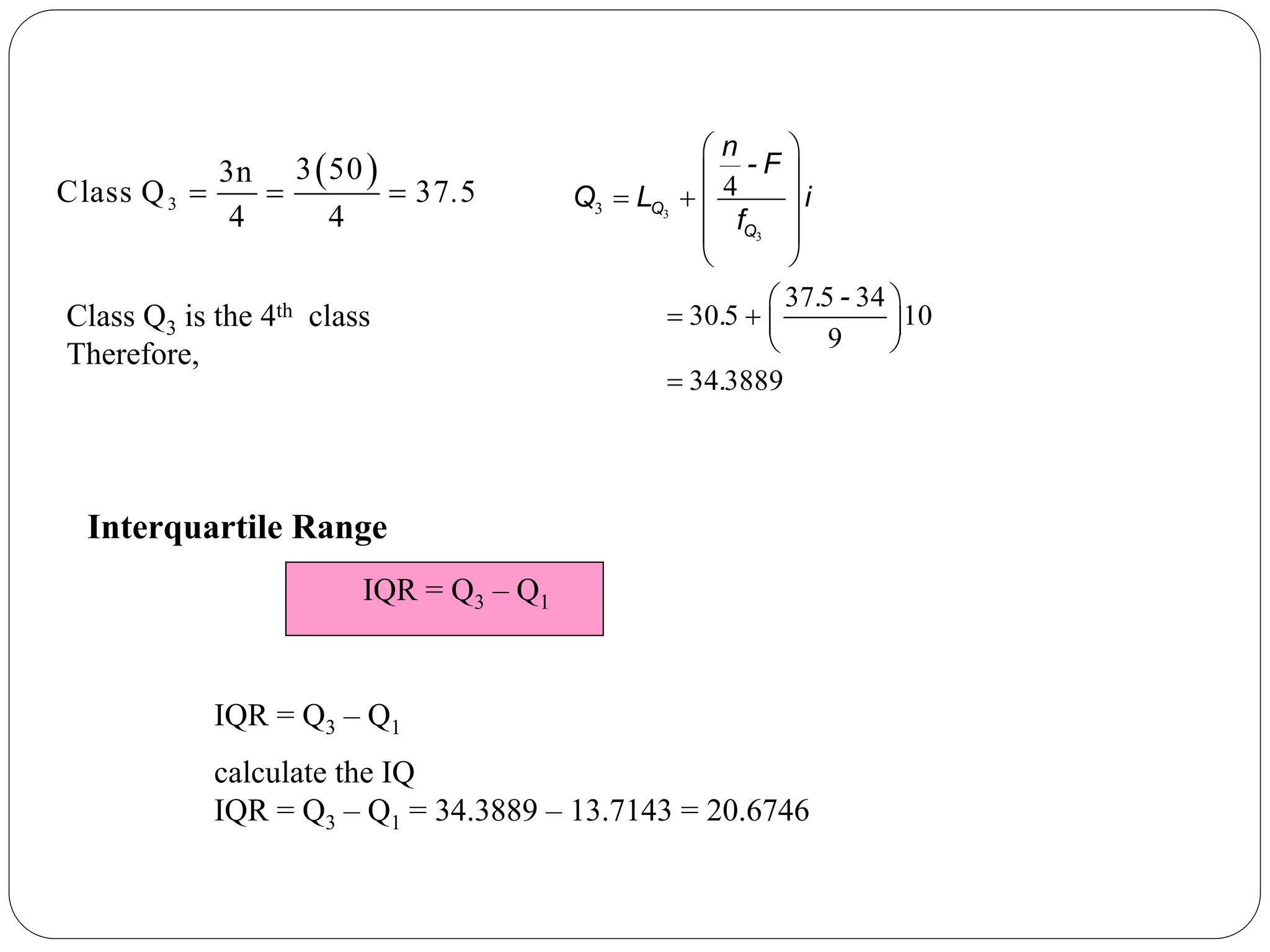
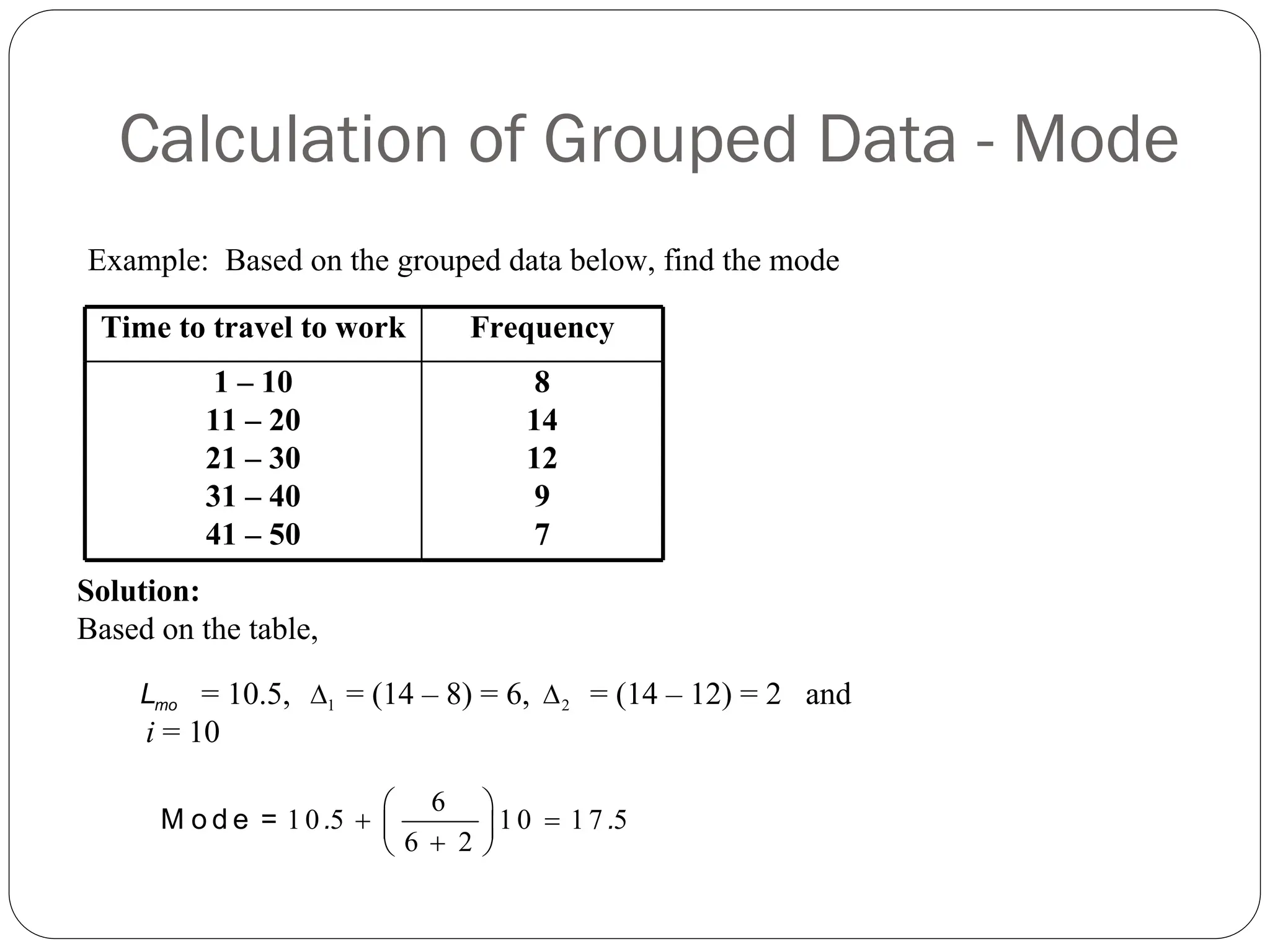
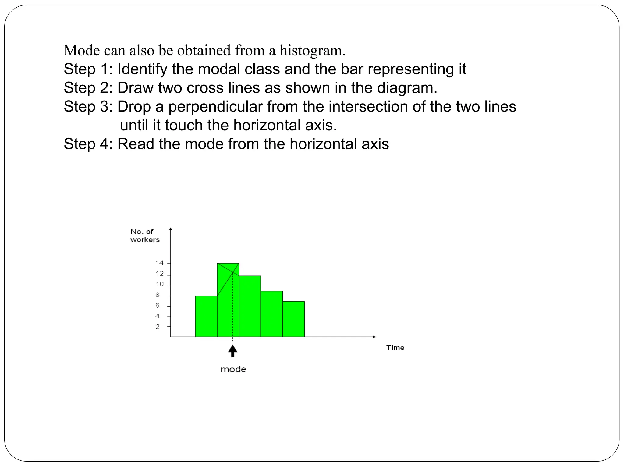
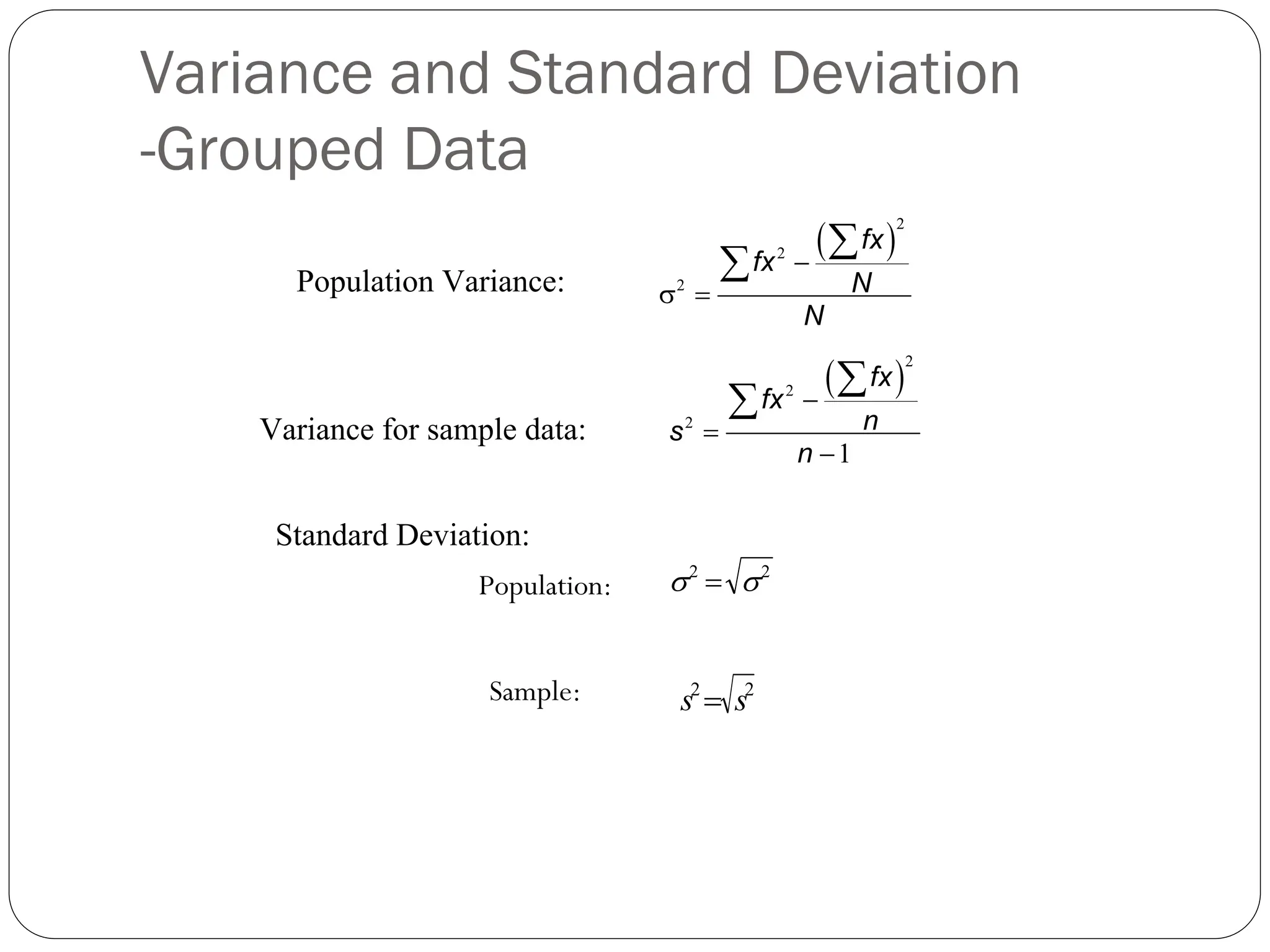
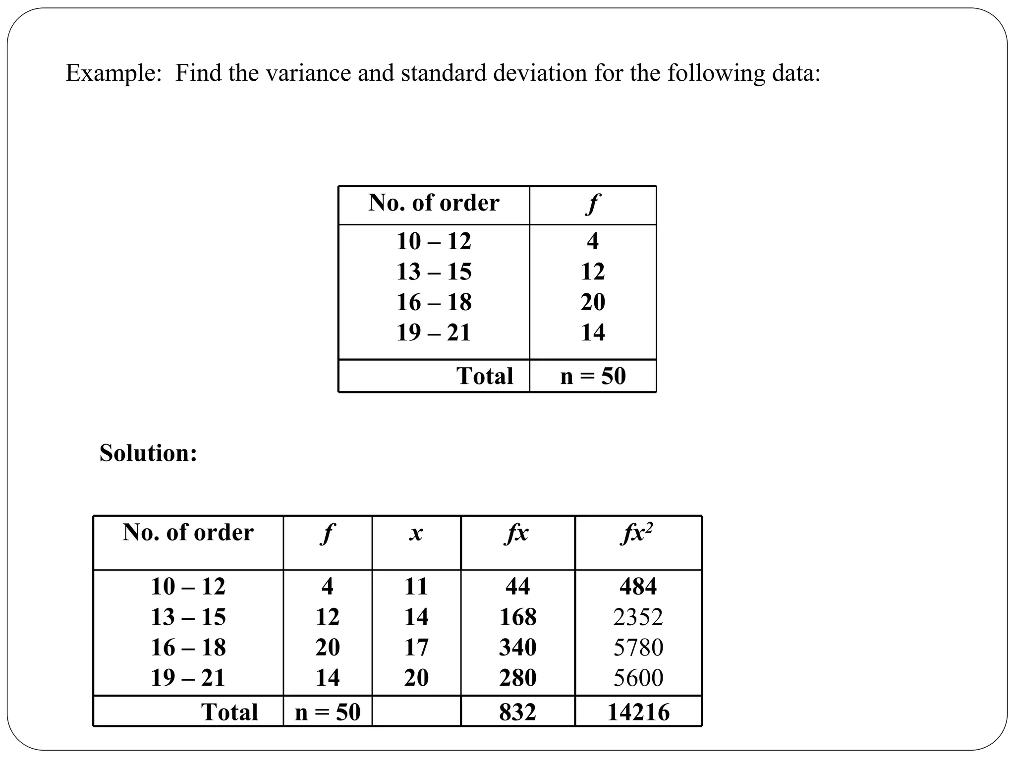
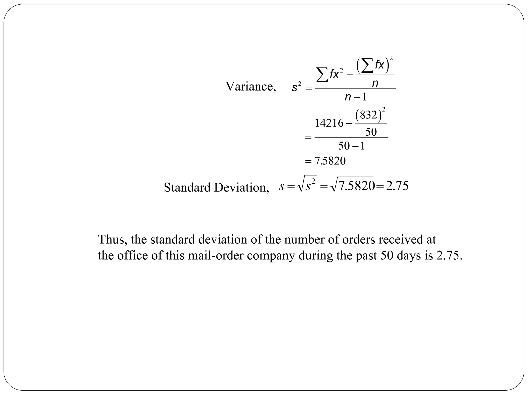
1. Mean, Median and Mode
2. First Quantile, third Quantile and
Interquantile Range.
Lecture 2 – Grouped Data
Calculation
Mean – Grouped Data
Number
of order
f
10 – 12
13 – 15
16 – 18
19 – 21
4
12
20
14
n = 50
Number
of order
f x fx
10 – 12
13 – 15
16 – 18
19 – 21
4
12
20
14
11
14
17
20
44
168
340
280
n = 50 = 832
fx 832
x = = = 16.64
n 50
∑
Example: The following table gives the frequency distribution of the number
of orders received each day during the past 50 days at the office of a mail-order
company. Calculate the mean.
Solution:
X is the midpoint of the
class. It is adding the class
limits and divide by 2.
Median and Interquartile Range
– Grouped Data
Step 1: Construct the cumulative frequency distribution.
Step 2: Decide the class that contain the median.
Class Median is the first class with the value of cumulative
frequency equal at least n/2.
Step 3: Find the median by using the following formula:
M e d ia n
⎛ ⎞
⎜ ⎟
⎜ ⎟
⎜ ⎟
⎝ ⎠
m
m
n
- F
2
= L + i
f
m
L
m
f
Where:
n = the total frequency
F = the cumulative frequency before class median
i = the class width
= the lower boundary of the class median
= the frequency of the class median
Time to travel to work Frequency
1 – 10
11 – 20
21 – 30
31 – 40
41 – 50
8
14
12
9
7
Example: Based on the grouped data below, find the median:
Solution:
Time to travel
to work
Frequency Cumulative
Frequency
1 – 10
11 – 20
21 – 30
31 – 40
41 – 50
8
14
12
9
7
8
22
34
43
50
25
2
50
2
=
=
n
m
f m
L
1st Step: Construct the cumulative frequency distribution
class median is the 3rd class
So, F = 22, = 12, = 20.5 and i = 10
Therefore,
2
25 22
21 5 10
12
24
⎛ ⎞
⎜ ⎟
+ ⎜ ⎟
⎜ ⎟
⎝ ⎠
⎛ ⎞
+ ⎜ ⎟
⎝ ⎠
Median
=
=
m
m
n
- F
= L i
f
-
.
Thus, 25 persons take less than 24 minutes to travel to work and another 25 persons
take more than 24 minutes to travel to work.
1
1
1 Q
Q
n
- F
4
Q L + i
f
⎛ ⎞
⎜ ⎟
= ⎜ ⎟
⎜ ⎟
⎝ ⎠
⎛ ⎞
⎜ ⎟
= ⎜ ⎟
⎜ ⎟
⎝ ⎠
3
3
3 Q
Q
3 n
- F
4
Q L + i
f
Quartiles
Using the same method of calculation as in the Median,
we can get Q1 and Q3 equation as follows:
Time to travel to work Frequency
1 – 10
11 – 20
21 – 30
31 – 40
41 – 50
8
14
12
9
7
Example: Based on the grouped data below, find the Interquartile Range
Time to travel
to work
Frequency Cumulative
Frequency
1 – 10
11 – 20
21 – 30
31 – 40
41 – 50
8
14
12
9
7
8
22
34
43
50
1
n 50
Class Q 12 5
4 4
.
= = =
1
1
1
4
12 5 8
10 5 10
14
13 7143
⎛ ⎞
⎜ ⎟
= + ⎜ ⎟
⎜ ⎟
⎝ ⎠
⎛ ⎞
= + ⎜ ⎟
⎝ ⎠
=
Q
Q
n
- F
Q L i
f
. -
.
.
Solution:
1st Step: Construct the cumulative frequency distribution
Class Q1 is the 2nd class
Therefore,
2nd Step: Determine the Q1 and Q3
( )
3
3 50
3n
Class Q 37 5
4 4
.
= = =
3
3
3
4
37 5 34
30 5 10
9
34 3889
⎛ ⎞
⎜ ⎟
= + ⎜ ⎟
⎜ ⎟
⎝ ⎠
⎛ ⎞
= + ⎜ ⎟
⎝ ⎠
=
Q
Q
n
- F
Q L i
f
. -
.
.
IQR = Q3 – Q1
Class Q3 is the 4th class
Therefore,
Interquartile Range
IQR = Q3 – Q1
calculate the IQ
IQR = Q3 – Q1 = 34.3889 – 13.7143 = 20.6746
Mode
•Mode is the value that has the highest frequency in a data set.
•For grouped data, class mode (or, modal class) is the class with the highest frequency.
•To find mode for grouped data, use the following formula:
⎛ ⎞
⎜ ⎟
⎝ ⎠
M o d e 1
m o
1 2
Δ
= L + i
Δ + Δ
Mode – Grouped Data
mo
L
1
Δ
2
Δ
Where:
is the lower boundary of class mode
is the difference between the frequency of class mode
and the frequency of the class before the class mode
is the difference between the frequency of class mode and the frequency
of the class after the class mode
i is the class width
Calculation of Grouped Data - Mode
Time to travel to work Frequency
1 – 10
11 – 20
21 – 30
31 – 40
41 – 50
8
14
12
9
7
Example: Based on the grouped data below, find the mode
mo
L 1
Δ 2
Δ
6
1 0 5 1 0 1 7 5
6 2
⎛ ⎞
+ =
⎜ ⎟
+
⎝ ⎠
M o d e = . .
Solution:
Based on the table,
= 10.5, = (14 – 8) = 6, = (14 – 12) = 2 and
i = 10
Mode can also be obtained from a histogram.
Step 1: Identify the modal class and the bar representing it
Step 2: Draw two cross lines as shown in the diagram.
Step 3: Drop a perpendicular from the intersection of the two lines
until it touch the horizontal axis.
Step 4: Read the mode from the horizontal axis
( )
2
2
2
−
σ =
∑
∑
fx
fx
N
N
( )
2
2
2
1
−
=
−
∑
∑
fx
fx
n
s
n
2
2
σ
σ =
2
2
s
s =
Population Variance:
Variance for sample data:
Standard Deviation:
Population:
Sample:
Variance and Standard Deviation
-Grouped Data
No. of order f
10 – 12
13 – 15
16 – 18
19 – 21
4
12
20
14
Total n = 50
No. of order f x fx fx2
10 – 12
13 – 15
16 – 18
19 – 21
4
12
20
14
11
14
17
20
44
168
340
280
484
2352
5780
5600
Total n = 50 832 14216
Example: Find the variance and standard deviation for the following data:
Solution:
( )
( )
2
2
2
2
1
832
14216
50
50 1
7 5820
−
=
−
−
=
−
=
∑
∑
fx
fx
n
s
n
.
75
.
2
5820
.
7
2
=
=
= s
s
Variance,
Standard Deviation,
Thus, the standard deviation of the number of orders received at
the office of this mail-order company during the past 50 days is 2.75.

Grouped Data Calculation type of data .pdf

  • 1.
    1. Mean, Medianand Mode 2. First Quantile, third Quantile and Interquantile Range. Lecture 2 – Grouped Data Calculation
  • 2.
    Mean – GroupedData Number of order f 10 – 12 13 – 15 16 – 18 19 – 21 4 12 20 14 n = 50 Number of order f x fx 10 – 12 13 – 15 16 – 18 19 – 21 4 12 20 14 11 14 17 20 44 168 340 280 n = 50 = 832 fx 832 x = = = 16.64 n 50 ∑ Example: The following table gives the frequency distribution of the number of orders received each day during the past 50 days at the office of a mail-order company. Calculate the mean. Solution: X is the midpoint of the class. It is adding the class limits and divide by 2.
  • 3.
    Median and InterquartileRange – Grouped Data Step 1: Construct the cumulative frequency distribution. Step 2: Decide the class that contain the median. Class Median is the first class with the value of cumulative frequency equal at least n/2. Step 3: Find the median by using the following formula: M e d ia n ⎛ ⎞ ⎜ ⎟ ⎜ ⎟ ⎜ ⎟ ⎝ ⎠ m m n - F 2 = L + i f m L m f Where: n = the total frequency F = the cumulative frequency before class median i = the class width = the lower boundary of the class median = the frequency of the class median
  • 4.
    Time to travelto work Frequency 1 – 10 11 – 20 21 – 30 31 – 40 41 – 50 8 14 12 9 7 Example: Based on the grouped data below, find the median: Solution: Time to travel to work Frequency Cumulative Frequency 1 – 10 11 – 20 21 – 30 31 – 40 41 – 50 8 14 12 9 7 8 22 34 43 50 25 2 50 2 = = n m f m L 1st Step: Construct the cumulative frequency distribution class median is the 3rd class So, F = 22, = 12, = 20.5 and i = 10
  • 5.
    Therefore, 2 25 22 21 510 12 24 ⎛ ⎞ ⎜ ⎟ + ⎜ ⎟ ⎜ ⎟ ⎝ ⎠ ⎛ ⎞ + ⎜ ⎟ ⎝ ⎠ Median = = m m n - F = L i f - . Thus, 25 persons take less than 24 minutes to travel to work and another 25 persons take more than 24 minutes to travel to work.
  • 6.
    1 1 1 Q Q n - F 4 QL + i f ⎛ ⎞ ⎜ ⎟ = ⎜ ⎟ ⎜ ⎟ ⎝ ⎠ ⎛ ⎞ ⎜ ⎟ = ⎜ ⎟ ⎜ ⎟ ⎝ ⎠ 3 3 3 Q Q 3 n - F 4 Q L + i f Quartiles Using the same method of calculation as in the Median, we can get Q1 and Q3 equation as follows: Time to travel to work Frequency 1 – 10 11 – 20 21 – 30 31 – 40 41 – 50 8 14 12 9 7 Example: Based on the grouped data below, find the Interquartile Range
  • 7.
    Time to travel towork Frequency Cumulative Frequency 1 – 10 11 – 20 21 – 30 31 – 40 41 – 50 8 14 12 9 7 8 22 34 43 50 1 n 50 Class Q 12 5 4 4 . = = = 1 1 1 4 12 5 8 10 5 10 14 13 7143 ⎛ ⎞ ⎜ ⎟ = + ⎜ ⎟ ⎜ ⎟ ⎝ ⎠ ⎛ ⎞ = + ⎜ ⎟ ⎝ ⎠ = Q Q n - F Q L i f . - . . Solution: 1st Step: Construct the cumulative frequency distribution Class Q1 is the 2nd class Therefore, 2nd Step: Determine the Q1 and Q3
  • 8.
    ( ) 3 3 50 3n ClassQ 37 5 4 4 . = = = 3 3 3 4 37 5 34 30 5 10 9 34 3889 ⎛ ⎞ ⎜ ⎟ = + ⎜ ⎟ ⎜ ⎟ ⎝ ⎠ ⎛ ⎞ = + ⎜ ⎟ ⎝ ⎠ = Q Q n - F Q L i f . - . . IQR = Q3 – Q1 Class Q3 is the 4th class Therefore, Interquartile Range IQR = Q3 – Q1 calculate the IQ IQR = Q3 – Q1 = 34.3889 – 13.7143 = 20.6746
  • 9.
    Mode •Mode is thevalue that has the highest frequency in a data set. •For grouped data, class mode (or, modal class) is the class with the highest frequency. •To find mode for grouped data, use the following formula: ⎛ ⎞ ⎜ ⎟ ⎝ ⎠ M o d e 1 m o 1 2 Δ = L + i Δ + Δ Mode – Grouped Data mo L 1 Δ 2 Δ Where: is the lower boundary of class mode is the difference between the frequency of class mode and the frequency of the class before the class mode is the difference between the frequency of class mode and the frequency of the class after the class mode i is the class width
  • 10.
    Calculation of GroupedData - Mode Time to travel to work Frequency 1 – 10 11 – 20 21 – 30 31 – 40 41 – 50 8 14 12 9 7 Example: Based on the grouped data below, find the mode mo L 1 Δ 2 Δ 6 1 0 5 1 0 1 7 5 6 2 ⎛ ⎞ + = ⎜ ⎟ + ⎝ ⎠ M o d e = . . Solution: Based on the table, = 10.5, = (14 – 8) = 6, = (14 – 12) = 2 and i = 10
  • 11.
    Mode can alsobe obtained from a histogram. Step 1: Identify the modal class and the bar representing it Step 2: Draw two cross lines as shown in the diagram. Step 3: Drop a perpendicular from the intersection of the two lines until it touch the horizontal axis. Step 4: Read the mode from the horizontal axis
  • 12.
    ( ) 2 2 2 − σ = ∑ ∑ fx fx N N () 2 2 2 1 − = − ∑ ∑ fx fx n s n 2 2 σ σ = 2 2 s s = Population Variance: Variance for sample data: Standard Deviation: Population: Sample: Variance and Standard Deviation -Grouped Data
  • 13.
    No. of orderf 10 – 12 13 – 15 16 – 18 19 – 21 4 12 20 14 Total n = 50 No. of order f x fx fx2 10 – 12 13 – 15 16 – 18 19 – 21 4 12 20 14 11 14 17 20 44 168 340 280 484 2352 5780 5600 Total n = 50 832 14216 Example: Find the variance and standard deviation for the following data: Solution:
  • 14.
    ( ) ( ) 2 2 2 2 1 832 14216 50 501 7 5820 − = − − = − = ∑ ∑ fx fx n s n . 75 . 2 5820 . 7 2 = = = s s Variance, Standard Deviation, Thus, the standard deviation of the number of orders received at the office of this mail-order company during the past 50 days is 2.75.