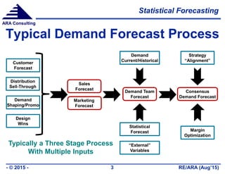
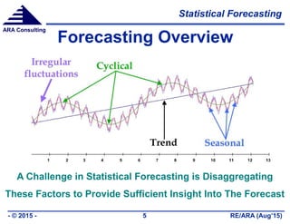
The document discusses statistical forecasting in the semiconductor industry, emphasizing the importance of custom models for accurate demand prediction. It outlines the typical processes, challenges, and capabilities required for effective forecasting, including the role of historical data, seasonality, and causal factors. Additionally, it introduces demand signal forecasting (DSF) as a method to enhance forecasting accuracy by integrating customer backlog and other leading indicators.

1. ARA Consulting
Statistical Forecasting
August’15- © 2015 - 1
ARA Consulting
Semiconductor Industry
Demand Forecasting Using
Custom Models
Russ / Tony 5/28/2015
Russ Elias
Tony Alvarez
June 2015Russ Elias
Tony Alvarez

2. Statistical Forecasting
RE/ARA (Aug’15)- © 2015 - 2
ARA Consulting
If You Forecast Like Everyone Else
You’ll Get The Same Results That
Everyone Else Gets

3. Statistical Forecasting
RE/ARA (Aug’15)- © 2015 - 3
ARA Consulting
Typical Demand Forecast Process
Customer
Forecast
Statistical
Forecast
Distribution
Sell-Through
Design
Wins
“External”
Variables
Demand
Current/Historical
Margin
Optimization
Strategy
“Alignment”
Demand
Shaping/Promo
Demand Team
Forecast
Consensus
Demand Forecast
Sales
Forecast
Marketing
Forecast
Typically a Three Stage Process
With Multiple Inputs

4. Statistical Forecasting
RE/ARA (Aug’15)- © 2015 - 4
ARA Consulting
Forecasting Overview
Forecast = Trendt-1 + Seasonalityt-1 + Cyclicalt-1 + Irregularitiest-1 +
Causal Factor(s) + Random (Unexplained) Variation
Trend Seasonality
Cyclical Irregular
Time
Time
Time
Causal
X1
Time

5. Statistical Forecasting
RE/ARA (Aug’15)- © 2015 - 5
ARA Consulting
A Challenge in Statistical Forecasting is Disaggregating
These Factors to Provide Sufficient Insight Into The Forecast
Forecasting Overview

6. Statistical Forecasting
RE/ARA (Aug’15)- © 2015 - 6
ARA Consulting
Typical Progression
No Seasonality
or
Trends?
Trends
But
No Seasonality?
Trends
&
Seasonality?
Trends, Seasonality
&
Causal Factors?
ARIMAX
Holts-Winters Smoothing
(Multiplicative & Additive)
or ARIMA
Holt’s Linear Method
(Double Exponential Smoothing)
Simple (Single) Exponential Smoothing
(Filters Noise/Irregularities)

7. Statistical Forecasting
RE/ARA (Aug’15)- © 2015 - 7
ARA Consulting
Basic Capabilities Required
 Level 1: Limiting & Damping, Seasonal Smoothing, Demand
Filtering, Reasonability Tests
 Level 2: Seasonal-with-Trend, Moving Average and Low-level
Pattern Fitting
 Level 3A: Trend Models For Products With Sporadic, Low-
Volume Demand
 Level 3B: Weighting of Historical Demand Seasonality; But
“System Doesn’t Know It’s Christmas Until It Sees It Twice.”
 Level 3C: Outlier Detection (Irregular Events); Determining
Which Elements Are Anomalous and Should Be Filtered

8. Statistical Forecasting
RE/ARA (Aug’15)- © 2015 - 8
ARA Consulting
“Boxed” Forecasting Software
 Typical Sequence
1)Product History Analyzed Using Variety (Dozens!) of Algorithms
2)Automatically Selects Best Algorithm For Each Product
3)Selection Based on How Well Algorithm Fits Historical Product Data
4)Winning Algorithm Used to Project Future Sales
 Forecasting Algorithm Will Always Produce Fcst; But
That Fcst Won’t Always Be a Good One
 “Over-Fitting” – Occurs When “Fit Noise in Data Rather
Than Discovering Underlying Structure”
 Pick Model That is Most Appropriate For Good Fcst;
May Not Be Model That “Best” Fits Historical Data

9. Statistical Forecasting
RE/ARA (Aug’15)- © 2015 - 9
ARA Consulting
That’s What You Get From “Boxed”
Solutions in Typical Forecasting
Packages
What’s Missing?

10. Statistical Forecasting
RE/ARA (Aug’15)- © 2015 - 10
ARA Consulting
Forecast Out of the Box!
Wealth of Information
Beyond Historical Product Data

11. Statistical Forecasting
RE/ARA (Aug’15)- © 2015 - 11
ARA Consulting
Application of Custom Models For
Semiconductor Forecasting
Data Typically Available:
Historical Product Demand & Delivery Data
Product Inventory Levels
Product Delinquency
Specific End-Market Forecasts
General Macro-Economic Trends
Customer Product Backlog

12. Statistical Forecasting
RE/ARA (Aug’15)- © 2015 - 12
ARA Consulting
Application of DSF For
Semiconductor Forecasting
 Demand Signal Forecasting (DSF)
• Forward-Looking Approach to Custom Models
• Utilizes Customer Backlog (VOC) as a Leading Indictor to
Augment Historical Data
• But, Customer Backlog Lead Time is Typically Less That What is
Required to Initiate Product Builds – Need ‘Gap Fill’ Forecast
 Demand Signal Forecasting (DSF) + Indicator Variables
• Can Further Customize Model By Incorporating Indicator Variables
• Example: Inventory Levels, Delinquency, End-Market Forecasts,
and Macro-Economic Trends to Further Refine & Customize Model

13. Statistical Forecasting
RE/ARA (Aug’15)- © 2015 - 13
ARA Consulting
DSF Application Example
 Background
• Customer’s Backlog is Often a Weak Forward Looking Signal Beyond One
Month; i.e. 30 Day Backlog Usually Reliable, 60 and 90 Day Backlog
Usually Subject to Significant Changes
• Manufacturing Cycle Times Range From ~90 Days (Si Start to Ship) to 15
– 30 Days (Wafer Bank to Ship)
• Mis-Match Between Backlog Signal Timing & Mfg Cycle Time Can Be
Managed With Inventory Staging, But at a Cost
• But, Tradeoff Inventory Risk vs. Customer Delinquency/Satisfaction
 Demand Signal Forecasting Generations
• Gen 1: Backlog as Leading Indicator Variable (Elias 2000 Thesis)
• Gen 2: Mid-Range Backlog Imputation in a Transfer Function Based
Custom Model to Create a Better Leading Indicator (Elias and Alvarez,
2014 Unpublished Work)
 DSF Gen 2 Addresses Mis-Match Between Customer Backlog
Timing as a Useful Leading Indicator & Mfg Cycle Time

14. Statistical Forecasting
RE/ARA (Aug’15)- © 2015 - 14
ARA Consulting
D = Demand
C = Custom DSF2
E = EWMA
DSF2 Applied to High Volume Consumer Product
• One Product
• One Customer
• One Market Segment

15. Statistical Forecasting
RE/ARA (Aug’15)- © 2015 - 15
ARA Consulting
DSF2 Model Results
D = Demand
C = Custom DSF2
e = Error

16. Statistical Forecasting
RE/ARA (Aug’15)- © 2015 - 16
ARA Consulting
DSF Gen 2 – First Step
0
0.1
0.2
0.3
0.4
1 2 3 4 5 6 7
Weighting by Age
DSF2 Looks Backward and Develops
Optimal ARIMA Model Based on Past
Demand and Past Forecast Errors

17. Statistical Forecasting
RE/ARA (Aug’15)- © 2015 - 17
ARA Consulting
DSF Gen 2 – Second Step
DSF2 Then Looks Forward and Uses a
Transfer Function to Blend in Backlog
0
0.2
0.4
1 2 3 4 5 6 7
Weighting by Age
Backlog
0
0.2
0.4
1 2 3 4 5 6 7
Weighting by Age
forecasts:
Yt+1, Yt+2, Yt+3
(Idealized)

18. Statistical Forecasting
RE/ARA (Aug’15)- © 2015 - 18
ARA Consulting
Forecast Benchmarks
 DSF2 Compared to Four Alternate Forecasting Methods:
• Exponentially Weighted Moving Averages (EWMA), with Automated
Smoothing Coefficient Optimization
• Holt-Winters Seasonal Decomposition
• Auto-Regressive Integrated Moving Average (ARIMA), with Monthly
MAPE-Optimal Model Parameterization
• Sales and Operational Planning (S&OP) Consensus Forecasting
 Forecast Methods Comparison Metrics:
• Bias % (Cum Actual – Cum Forecast)*100/Cum Actual
• Mean Absolute Percent Error (MAPE)
• Normalized Inventory Dollar Maximum Delinquency and Final Period
Delinquency or Inventory Level
• Forecast Performance Graphs Showing Head-to-Head Results

19. Statistical Forecasting
RE/ARA (Aug’15)- © 2015 - 19
ARA Consulting
Forecast Method Comparisons:
Statistical Metrics
Rank Method Bias MAPE
5 S&OP 58% 63%
4 EWMA -1.3% 55%
3 Holt-Winters -9.6% 42%
2 ARIMA -7.9% 34%
1 DSF Gen 2 4.3% 27%
The Custom DSF2 Model Outperformed Both the S&OP
Consensus Forecast and the Conventional Statistical Models
Available in Demand Planning Software Packages
Interesting, But Where’s The Money?

20. Statistical Forecasting
RE/ARA (Aug’15)- © 2015 - 20
ARA Consulting
Forecast Method Comparisons:
Financial Metrics
Rank Method
Max
Delinquency
Period End Inventory
or (Delinquency)
Period End
Months Inventory
5 S&OP $17M ($14M) n/a
4 EWMA $9.5M $12M 6 Months
3 Holt-Winters $3M $14M 7 Months
2 ARIMA $2M $11M 5.5 Months
1 DSF Gen 2 $3M $3M 1.5 Months
Bottom Line High ROI:
Less Delinquency/Missed Sales & Higher Customer Satisfaction
Less Inventory Build/Working Capital, Reduced Inventory Exposure
In Reality Implications More Severe as Assumed that 100% of Delinquency
‘Catch-up’ Builds are Sold; Typically Some Portion Gets Cancelled Resulting in
Lost Sales and Therefore Even More Excess Inventory
Note: Semiconductor Industry ASP ~$1.25, For Illustrative Purposed Normalized Unit ASP Set to $1 and Normalized Units to 1M/Month

21. Statistical Forecasting
RE/ARA (Aug’15)- © 2015 - 21
ARA Consulting
D = Demand
C = Custom DSF2
E = EWMA
DSF2 vs. EWMA Forecast

22. Statistical Forecasting
RE/ARA (Aug’15)- © 2015 - 22
ARA Consulting
D = Demand
C = Custom DSF2
H = Holt-Winters
DSF2 vs. Holt-Winters Forecast

23. Statistical Forecasting
RE/ARA (Aug’15)- © 2015 - 23
ARA Consulting
D = Demand
C = Custom DSF2
A = ARIMA
DSF2 vs. ARIMA Forecast

24. Statistical Forecasting
RE/ARA (Aug’15)- © 2015 - 24
ARA Consulting
D = Demand
C = Custom DSF2
S = S&OP Fcst
DSF2 vs. S&OP Lead 3 Forecast

25. Statistical Forecasting
RE/ARA (Aug’15)- © 2015 - 25
ARA Consulting
Inventory Observations
S&OP: Keeps Predicting Product’s Demise – Never Caught Up With Demand
EWMA: Slow to Respond - Initially Delinquent Then Over-Builds
Holt-Winters: Moderate Bullwhip Effect Evident – Builds-Delinquent-Builds
ARIMA: Starts Off Reasonably, Doesn’t Respond to Final Rapid Drop
DSF2: Starts Off Reasonably, By Utilizing Customer Backlog Keeps From Overbuilding
Delinquent Supply
Excess Inventory

26. Statistical Forecasting
RE/ARA (Aug’15)- © 2015 - 26
ARA Consulting
Conclusion
Forecasting System Designed to Quickly Track Changes in Behavior
Can Create “Noisy” Forecasts During Periods of Relative Stability
Forecasting System Designed to Give Smooth Forecasts Will
Typically Lag True Changes
If Only Looking Back, There is No Reliable Way to Forecast What Will
Happen When Established Patterns or Relationships Change
It Follows That Without Forward Looking Data/Information,
Quantitative Methods & Corresponding Predictions are Only as
Reliable as The Stability of Patterns Modeled in Their Past History
This is Where Demand-Signal Forecasting
Comes In

27. Statistical Forecasting
RE/ARA (Aug’15)- © 2015 - 27
ARA Consulting
Caveats
Keep Modeling Approach “As Simple as Possible, But Not Simpler”
Custom Models Take Work, The DSF2 Model in This Example Took
~40 Hrs Hours to Develop & 1 Hr/Mth Maintenance
While Modest Within Overall Costs Associated With an S&OP Effort
and Very High ROI, the Optimal Method Depends on The Situation
DSF2 Was The Optimal Approach in This Example (And Others), But
That Will Not Be True in All Situations
In Course of This Work, Multiple Custom Models Were Utilized For
Different Products; In All But One Case The Statistical Models Out-
Performed the S&OP Consensus Forecast
DSF2 Works Best When Customer Order Patterns are Subject to
Rapid Changes and Historical Data is Insufficient to Provide a Good
Predictor of the Future
Therefore, ….

28. Statistical Forecasting
RE/ARA (Aug’15)- © 2015 - 28
ARA Consulting
One Size Does Not
Fit All

29. Statistical Forecasting
RE/ARA (Aug’15)- © 2015 - 29
ARA Consulting
Optimal Forecasting Method Depends on
Many Variables
Segmentation Often Used to Match
Forecasting Method to Product Category
Best to Use Simplest/Lowest Cost
“Acceptable” Method (Forecast Value Add)

30. Statistical Forecasting
RE/ARA (Aug’15)- © 2015 - 30
ARA Consulting
Conventional Segmentation
Forecasting Technique vs. Product Category
(After Demand Driven Forecasting)

31. Statistical Forecasting
RE/ARA (Aug’15)- © 2015 - 31
ARA Consulting
Recommended Segmentation Variables:
Product Lifecycle Position
Volume (Pareto Principle)
Degree of Intermittency
Margin
Semiconductor Segmentation
Fast Ramp
Slow Ramp
Delayed Ramp
New Product Mid-Life Product
Top 20
Low Volume
Steady State
Fast Ramp
Slow Ramp
Controlled EOL
EOL Product
Low Volume
Intermittent
Build to
Order
(Lead Times
13 – 16
Weeks)
Low Margin

BTO
High Margin

Bank to Fcst
& FTO
Bank to Fcst
Finish to
Order (FTO)
(Lead Times
4– 6 Weeks)

32. Statistical Forecasting
RE/ARA (Aug’15)- © 2015 - 32
ARA Consulting
Recommended
Consider
Not Required or Inapplicable
When to Use Custom Model
Fast Ramp
Slow Ramp
Delayed Ramp
New Product Mid-Life Product
Top 20
Low Volume
Steady State
Fast Ramp
Slow Ramp
Controlled EOL
EOL Product
Low Volume
Intermittent
Build to
Order
(Lead Times
13 – 16
Weeks)
Low Margin

BTO
High Margin

Bank to Fcst
& FTO
Bank to Fcst
Finish to
Order (FTO)
(Lead Times
4– 6 Weeks)

33. Statistical Forecasting
RE/ARA (Aug’15)- © 2015 - 33
ARA Consulting
Top “20”
Typically 50 – 80% of a Company’s or Business Unit’s Revenue
Bank to Fcst: Custom Models Worth The Effort; Heuristics Need to Be Understood
Finish to Order (FTO): Theoretically No Fcst Required; Lead 1 Backlog Could be Used to
Aid Decision Making When Order “Smoothing” Required for Production Purposes
Semiconductor Segmentation
Fast Ramp
Slow Ramp
Delayed Ramp
New Product Mid-Life Product
Top 20
Low Volume
Steady State
Fast Ramp
Slow Ramp
Controlled EOL
EOL Product
Low Volume
Intermittent
Build to
Order
(Lead Times
13 – 16
Weeks)
Low Margin

BTO
High Margin

Bank to Fcst
& FTO
Bank to Fcst
Finish to
Order (FTO)
(Lead Times
4– 6 Weeks)

34. Statistical Forecasting
RE/ARA (Aug’15)- © 2015 - 34
ARA Consulting
Low Volume Steady State
High Margin: Consider Custom Models as Necessary; Could Be Very High ROI
“Boxed” Statistical Models May Be Acceptable (Low Effort) for Bank to Fcst
Low Margin: Build to Order (BTO)
Semiconductor Segmentation
Fast Ramp
Slow Ramp
Delayed Ramp
New Product Mid-Life Product
Top 20
Low Volume
Steady State
Fast Ramp
Slow Ramp
Controlled EOL
EOL Product
Low Volume
Intermittent
Build to
Order
(Lead Times
13 – 16
Weeks)
Low Margin

BTO
High Margin

Bank to Fcst
& FTO
Bank to Fcst
Finish to
Order (FTO)
(Lead Times
4– 6 Weeks)

35. Statistical Forecasting
RE/ARA (Aug’15)- © 2015 - 35
ARA Consulting
Low Volume Intermittent
Statistical Models Probably Won’t Work Well or Worth the Effort
Best to Keep as BTO
Semiconductor Segmentation
Fast Ramp
Slow Ramp
Delayed Ramp
New Product Mid-Life Product
Top 20
Low Volume
Steady State
Fast Ramp
Slow Ramp
Controlled EOL
EOL Product
Low Volume
Intermittent
Build to
Order
(Lead Times
13 – 16
Weeks)
Low Margin

FTO
High Margin

Bank to Fcst
FTO
Bank to Fcst
Finish to
Order (FTO)
(Lead Times
4– 6 Weeks)

36. Statistical Forecasting
RE/ARA (Aug’15)- © 2015 - 36
ARA Consulting
Treat Statistical Forecasting as a “Black Box” at
Your Peril
Understanding The Story Behind The Data is a
Requirement For Effective Forecasting
You Do Need to Understand the Heuristics
You Don’t Need to Understand the Computational
Details
Customized Demand Signal Forecasting
Model is Demonstrated to Provide
Significant Financial Benefit

37. Statistical Forecasting
RE/ARA (Aug’15)- © 2015 - 37
ARA Consulting
PDCA: Demand Forecasting
Plan
(Methods & Data)
Do
(Forecast Compilation)
Check
(Team Review)
Act
(Adjust & Learn)

38. Statistical Forecasting
RE/ARA (Aug’15)- © 2015 - 38
ARA Consulting
Appendix

39. Statistical Forecasting
RE/ARA (Aug’15)- © 2015 - 39
ARA Consulting
Approaches to Forecasting
Three Categories of Forecasting Models
(Logility – Seven Methods That Improve Forecast Accuracy)

40. Statistical Forecasting
RE/ARA (Aug’15)- © 2015 - 40
ARA Consulting
 ARIMA = Auto Regressive Integrated Moving Average
 ARIMAX
 ARIMA + eXogenous variables
 Advanced Statistical Algorithm That Produces Forecasts
Based Upon Weighted Nonlinear Combinations of Past
Realizations, Past Errors, and Future Leading Indicators
 Let’s Look at ARIMA a more in Detail ...
Custom Modeling Background

41. Statistical Forecasting
RE/ARA (Aug’15)- © 2015 - 41
ARA Consulting
ARIMA Looks at These Two Series:
1. The past demand values (D)
2. The past forecast error values (e)
Future Forecasts Are Weighted Combinations of
Past Values of These Two Series ... How It Weights
These Values is The Trick
D = Demand
e = Error
normalizedunits/month

42. Statistical Forecasting
RE/ARA (Aug’15)- © 2015 - 42
ARA Consulting
Rolling Average Weighting
 ARIMA Makes Future Predictions Based Upon Weighted
Combinations of Past Values
 Let’s Explore Weighting Options...
 A Rolling Average Weights Past Predictions Based Upon Equal
Weights of Past Observations:
0
0.2
0.4
1 2 3 4 5 6 7
Weighting by Age
age weight
1 0.25
2 0.25
3 0.25
4 0.25
5 0
6 0
7 0

43. Statistical Forecasting
RE/ARA (Aug’15)- © 2015 - 43
ARA Consulting
EWMA Weighting
 An Exponentially Weighted Moving Average (EWMA) Weights Past
Predictions Based Upon Weights That Follow an Exponentially Decaying
Value
 Weights Can Be Tuned By Selection of Decay Factor, But They Must
Always Be Monotonically Decreasing With Age Of Observation
0
0.05
0.1
0.15
0.2
1 2 3 4 5 6 7
Weighting by Ageage weight
1 0.16
2 0.128
3 0.1024
4 0.08192
5 0.065536
6 0.052429
7 0.041943

44. Statistical Forecasting
RE/ARA (Aug’15)- © 2015 - 44
ARA Consulting
ARIMA Weighting
 An Autoregressive Integrated Moving Average (ARIMA) Weights Past
Observations and Past Forecast Errors Based Upon Weights That Are
Calculated From Maximum Likelihood Estimation (MLE) Criteria
 This Permits Weights to Assume Any Values Required; Constrained Only to
Sum to Unity
 ARIMA’s Use of MLE For Parameter Estimation Gives it Theoretical
Statistical Optimality Qualities That EWMA and Holt-Winters Do Not Have
0
0.1
0.2
0.3
0.4
1 2 3 4 5 6 7
Weighting by Age
age weight
1 0.25
2 0.14
3 0.38
4 0.07
5 0.04
6 0.09
7 0.03