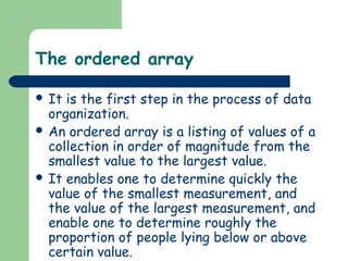
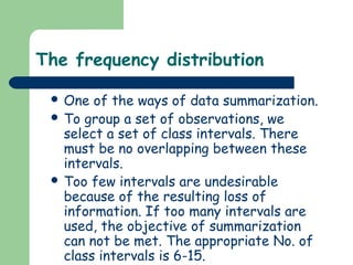
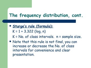
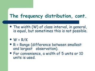
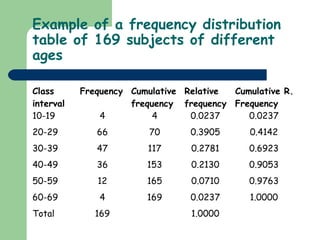
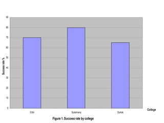
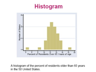
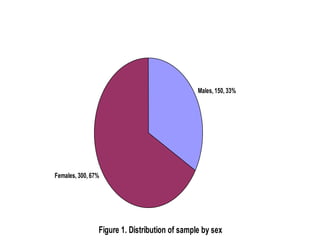
The document discusses methods for organizing and summarizing data, including ordered arrays, frequency distributions, and data visualization. It explains that an ordered array lists values from smallest to largest, and a frequency distribution groups data into class intervals to summarize observations. Guidelines are provided for determining the appropriate number of class intervals. Examples demonstrate a frequency distribution table and graphs, including a bar graph comparing college success rates, a histogram of ages, and a pie chart dividing a sample by sex.

1. Data presentation
Prepared by
Assis. Prof.
Namir G. Al-Tawil

2. The ordered array
 It is the first step in the process of data
organization.
 An ordered array is a listing of values of a
collection in order of magnitude from the
smallest value to the largest value.
 It enables one to determine quickly the
value of the smallest measurement, and
the value of the largest measurement, and
enable one to determine roughly the
proportion of people lying below or above
certain value.

6. The frequency distribution
 One of the ways of data summarization.
 To group a set of observations, we
select a set of class intervals. There
must be no overlapping between these
intervals.
 Too few intervals are undesirable
because of the resulting loss of
information. If too many intervals are
used, the objective of summarization
can not be met. The appropriate No. of
class intervals is 6-15.

7. The frequency distribution, cont.
 Sturge’s rule (formula):
K = 1 + 3.322 (log10 n)
K = No. of class intervals. n = sample size.
 Note that this rule is not final, you can
increase or decrease the No. of class
intervals for convenience and clear
presentation.

8. The frequency distribution, cont.
 The width (W) of class interval, in general,
is equal, but sometimes this is not possible.
W = R/K
 R = Range (difference between smallest
and largest observation).
 For convenience, a width of 5 units or 10
units is used.

9. Example of a frequency distribution
table of 169 subjects of different
ages
Class Frequency Cumulative Relative Cumulative R.
interval frequency frequency Frequency
10-19 4 4 0.0237 0.0237
20-29 66 70 0.3905 0.4142
30-39 47 117 0.2781 0.6923
40-49 36 153 0.2130 0.9053
50-59 12 165 0.0710 0.9763
60-69 4 169 0.0237 1.0000
Total 169 1.0000

14. 90
80
70
60
50
Success rate %
40
30
20
10
0
College
Erbil Sulaimany Duhok
Figure 1. Success rate by college

20. 6
5
4
frequency
3
2
1
0
17.5 20 22.5 25 27.5 30 32.5 35 37.5 40 42.5 45 47.5
Age (years)
The Frequency Polygon

21. 70
60
50
40
frequency
30
20
10
0
10 to 19 20 to 29 30 to 39 40 to 49 50 to 59 60 to 69
Distribution of Sample by Age Age (years)
Line Graph

22. Males, 150, 33%
Females, 300, 67%
Figure 1. Distribution of sample by sex