Download to read offline
![1
ES 128: Homework 2
Solutions
Problem 1
Show that the weak form of
02)( =+ x
dx
du
AE
dx
d
on 31 << x ,
1.0)1(
1
=
=
=xdx
du
Eσ ,
001.0)3( =u
is given by
∫∫ +−= =
3
1
1
3
1
2)(1.0 xwdxwAdx
dx
du
AE
dx
dw
x w∀ with 0)3( =w .
Solution
We multiply the governing equation and the natural boundary condition over the
domain [1, 3] by an arbitrary weight function:
02
3
1
=
+
∫ dxx
dx
du
AE
dx
d
w )(xw∀ , (1.1)
01.0
1
=
−
=x
dx
du
EwA )1(w∀ . (1.2)
We integrate (1.1) by parts as
dx
dx
du
AE
dx
dw
dx
du
wAEdx
dx
du
AE
dx
d
w
x
x
∫∫
−
=
=
=
3
1
3
1
3
1
. (1.3)
Substituting (1.3) into (1.1) gives
02
13
3
1
3
1
=
−
++
−
==
∫∫
xx
dx
du
wAE
dx
du
wAEwxdxdx
dx
du
AE
dx
dw
)(xw∀ . (1.4)
With 0)3( =w and 1.0)1( =σ , we obtain
( ) 1
3
1
3
1
1.02 =
−=
∫∫ x
wAwxdxdx
dx
du
AE
dx
dw
)(xw∀ with 0)3( =w . (1.5)](https://image.slidesharecdn.com/solutionhomework2-191026054137/85/Solution-homework2-1-320.jpg)
![1
ES 128: Homework 2
Solutions
Problem 1
Show that the weak form of
02)( =+ x
dx
du
AE
dx
d
on 31 << x ,
1.0)1(
1
=
=
=xdx
du
Eσ ,
001.0)3( =u
is given by
∫∫ +−= =
3
1
1
3
1
2)(1.0 xwdxwAdx
dx
du
AE
dx
dw
x w∀ with 0)3( =w .
Solution
We multiply the governing equation and the natural boundary condition over the
domain [1, 3] by an arbitrary weight function:
02
3
1
=
+
∫ dxx
dx
du
AE
dx
d
w )(xw∀ , (1.1)
01.0
1
=
−
=x
dx
du
EwA )1(w∀ . (1.2)
We integrate (1.1) by parts as
dx
dx
du
AE
dx
dw
dx
du
wAEdx
dx
du
AE
dx
d
w
x
x
∫∫
−
=
=
=
3
1
3
1
3
1
. (1.3)
Substituting (1.3) into (1.1) gives
02
13
3
1
3
1
=
−
++
−
==
∫∫
xx
dx
du
wAE
dx
du
wAEwxdxdx
dx
du
AE
dx
dw
)(xw∀ . (1.4)
With 0)3( =w and 1.0)1( =σ , we obtain
( ) 1
3
1
3
1
1.02 =
−=
∫∫ x
wAwxdxdx
dx
du
AE
dx
dw
)(xw∀ with 0)3( =w . (1.5)](https://image.slidesharecdn.com/solutionhomework2-191026054137/75/Solution-homework2-1-2048.jpg)
![2
El (1)
El (2)
1
2
3
Figure 1a
x
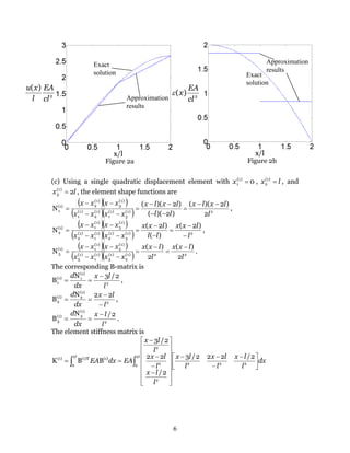
Problem 2
Consider the (steel) bar in Figure 1. The bar has
a uniform thickness t=1cm, Young’s modulus
E=200 9
10× Pa, and weight density
ρ =7 3
10× 3
/mkg . In addition to its self-weight,
the bar is subjected to a point load P=100N at
its midpoint.
(a) Model the bar with two finite elements.
(b) Write down expressions for the element
stiffness matrices and element body force
vectors.
(c) Assemble the structural stiffness matrix
K and global load vector F .
(d) Solve for the global displacement vector
d.
(e) Evaluate the stresses in each element.
(f) Determine the reaction force at the
support.
Solution
(a) Using two elements, each of 0.3m in length, we
obtain the finite element model in Figure 1a. In this
model, 0)1(
1 =x , 3.0)1(
2 =x , 3.0)2(
1 =x , 6.0)2(
2 =x ,
and A(x)=0.0012-0.001x .
(b) For element 1, [ ]xx−= 3.0
3.0
1
N(1)
,
[ ]11
3.0
1
B(1)
−= , the element stiffness matrix is
,
7.07.0
7.07.0
10
11
11
)001.00012.0(
09.0
10200
BBK
9
3.0
0
9
3.0
0
)1((1)T(1)
−
−
=
−
−
−
×
=
=
∫
∫
dxx
dxAE
the element body force vector is
( )
+
−
−−×
=
+=
∫
∫ =
100
0
)001.00012.0(
)001.00012.0)(3.0(
3.0
107
NNf
3.0
0
3
3.0
(1)T
3.0
0
(1)T(1)
dx
xx
xx
PAdx
x
ρ
=
05.101
155.1
, and the scatter matrix is
=
010
001
L(1)
.](https://image.slidesharecdn.com/solutionhomework2-191026054137/85/Solution-homework2-2-320.jpg)
![3
For element 2, [ ]3.06.0
3.0
1
N(2)
−−= xx , [ ]11
3.0
1
B(2)
−= , the element
stiffness matrix is
dxxdxAE ∫∫
−
−
−
×
==
6.0
3.0
9
6.0
3.0
)2((2)T(2)
11
11
)001.00012.0(
09.0
10200
BBK
,
5.05.0
5.05.0
109
−
−
= the element body force vector
is dx
xx
xx
Adx ∫∫
−−
−−×
==
6.0
3.0
3
6.0
3.0
(2)T(2)
)001.00012.0)(3.0(
)001.00012.0)(6.0(
3.0
107
Nf ρ =
735.0
84.0
, and
the scatter matrix is
=
100
010
L(2)
.
(c) The global stiffness matrix is
=+== ∑=
(2)(2)(2)T(1)(1)(1)T
2
1e
eeeT
LKLLKLLKLK
−
−−
−
5.05.00
5.02.17.0
07.07.0
109
.
The global load vector is
=+== ∑=
(2)(2)T(1)(1)T
2
1e
eeT
fLfLfLf
735.0
89.101
155.1
.
(d) Note that only the reaction force at node 1 is not zero, thus
+
=+
735.0
89.101
155.1
rf
1r
.
The resulting global system of equations is
−
−−
−
5.05.00
5.02.17.0
07.07.0
109
3
2
0
u
u =
+
735.0
89.101
155.11r
.
Solving the above equation,
2u = 1.46607 7_
10× (m), 3u = 1.48077 7_
10× (m), and 1r =-103.78(N).
(e) The stress field in element 1 is given by
×
−××== −7
9(1)(1))1(
1046607.1
0
]11[
3.0
1
10200dB)( Exσ =9.7738 4
10× (Pa).
The stress field in element 2 is given by
×
×
−××== −
−
7
7
9(2)(2))2(
1048077.1
1046607.1
]11[
3.0
1
10200dB)( Exσ =980 (Pa).
(f) The reaction force at the support Node 1 is -103.78N.](https://image.slidesharecdn.com/solutionhomework2-191026054137/85/Solution-homework2-3-320.jpg)
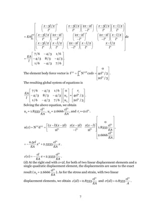
![4
Problem 3
Consider the mesh shown in Figure 2. The model consists of two linear
displacement constant strain elements. The cross-sectional area is A=1, Young’s
modulus is E; both are constant. A body force b(x)=cx is applied.
(a) Solve and plot u(x) and )(xε for
the FEM solution.
(b) Compare (by plotting) the finite
element solution against the exact
solution for the equation
.)(2
2
cxxb
dx
ud
E −=−=
(c) Solve the above problem using a single quadratic displacement element.
(d) Compare the accuracy of stress and displacement at the right end with that
of two linear displacement elements.
(e) Check whether the equilibrium equation and traction boundary condition
are satisfied for the two meshes.
Solution
(a) Using two linear displacement constant strain elements, each of l in length,
we obtain the finite element model with 0)1(
1 =x , lx =)1(
2 , lx =)2(
1 , and lx 2)2(
2 = .
For element 1, [ ]xxl
l
−=
1
N(1)
, [ ]11
1
B(1)
−=
l
, the element stiffness matrix is
−
−
=
11
11
K(1)
l
EA
, the element body force vector is
== ∫ 3/
6/
Nf 2
2
0
(1)T(1)
cl
cl
cxdx
l
,
and the scatter matrix is
=
010
001
L(1)
.
For element 2, [ ]lxxl
l
−−= 2
1
N(2)
, [ ]11
1
B(2)
−=
l
, the element stiffness matrix
is
−
−
=
11
11
K(2)
l
EA
, the element body force vector
is
== ∫ 6/5
3/2
Nf 2
2
2
(2)T(2)
cl
cl
cxdx
l
l
, and the scatter matrix is
=
100
010
L(2)
.
The global stiffness matrix is
=+== ∑=
(2)(2)(2)T(1)(1)(1)T
2
1e
eeeT
LKLLKLLKLK
−
−−
−
110
121
011
l
EA
.
The global load vector is
Figure 2](https://image.slidesharecdn.com/solutionhomework2-191026054137/85/Solution-homework2-4-320.jpg)
![5
=+== ∑=
(2)(2)T(1)(1)T
2
1e
eeT
fLfLfLf
8333.0
0.1
1667.0
2
cl .
The resulting global system of equations is
−
−−
−
110
121
011
l
EA
3
2
0
u
u =
+
2
2
2
1
8333.0
1667.0
cl
cl
clr
.
Solving the above equation,
2u = 1.8333
EA
cl3
, 3u = 2.6666
EA
cl3
, and 1r =-2 2
cl .
When lx ≤≤0
[ ]
EA
xcl
EA
clxxl
l
xu
2
3(1)(1)
8333.1
8333.1
01
dN)( =
−== ,
and
EA
cl
dx
du
x
2
8333.1)( ==ε .
When lxl 2≤≤
[ ] x
EA
cl
EA
cl
EA
cl
EA
cl
lxxl
l
xu
23
3
3
(2)(2)
8333.0
6666.2
8333.1
2
1
dN)( +=
−−== ,
and
EA
cl
dx
du
x
2
8333.0)( ==ε .
(b). The governing equation is
,)(2
2
cxxb
dx
ud
EA −=−=
where A=1. The boundary condition is u(0)=0, and 0)2( =lσ .
Solving this linear ODE, we obtain the exact solution 21
3
6
)( cxcx
EA
c
xu ++−= .
Since u(0)=0, 02 =c . Since 0)2( =lσ ,
EA
cl
c
2
1
2
= . Thus
x
EA
cl
x
EA
c
xu
2
3 2
6
)( +−= .
EA
cl
EA
cx
x
22
2
2
)( +−=ε
The comparisons between the approximation results and the exact solutions are
shown in Figures 2a (displacement), and 2b (strain).](https://image.slidesharecdn.com/solutionhomework2-191026054137/85/Solution-homework2-5-320.jpg)

The document provides solutions to three problems involving finite element analysis. Problem 1 shows the derivation of the weak form of a partial differential equation. Problem 2 sets up finite element models for a bar with two elements, assembles the stiffness matrix and load vector, and solves for displacements and stresses. Problem 3 models a problem with two linear elements, derives the finite element equations, and solves for displacements and stresses, then compares to an exact solution and a single quadratic element solution.