A Posteriori Error Analysis Presentation

A Posteriori Error Bound of DG in
Time and CG in Space FE Method for
Semilinear Parabolic Problems
Mohammad Sabawi
with
A. Cangiani and E. Georgoulis
Department of Mathematics
University of Leicester
February 20, 2015
FEM Workshop February 2015 A Posteriori EB of Time-DG and Space-CG FEM for SPPs

Outline
• Introduction
• Settings and Notations
• Fully discrete Case

Introduction
• The variational formulation of the DG
time stepping methods gives a ﬂexibility
in changing the time-steps and orders of
approximation and this allows for other
extensions such as hp-adaptivity.

• We derive a posteriori error bounds for semilinear
parabolic equation by using discontinuous Galerkin
method in time and continuous (conforming) ﬁnite
element in space. Our main tools in this analysis the
reconstruction in time and elliptic reconstruction in
space with Gronwall’s lemma and continuation
argument.

Advantages
• Strong stability properties.
• Flexibility in variation the size of time
steps and local orders of approximation
leading to hp-adaptivity.
• DG time-stepping methods with
appropriate quadrature are equivalent to
Runge-Kutta-Radau methods.

Disadvantages
• High eﬀort in implementation for higher
orders.
• High computational cost for solving large
linear systems with block matrices.

Literature Review
• Makridakis and Nochetto 2006, Derived a
posteriori bounds for the semidiscrete
case by deﬁning a novel higher order time
reconstruction.
• Sch¨otzau and Wihler 2010, derived a
posteriori bounds for hp-version DG by
using time reconstruction.
• Georgoulis, Lakkis and Wihler, Derived a
posteriori bounds for the fully discrete
linear parabolic equation by using time
reconstruction technique, in progress.

The Mathematical Model and Settings
We consider the following initial value semilinear
parabolic equation
u + Au = f (u), u(0) = u0 (1)
where A is the elliptic bounded self adjoint operator
A : V −→ V ∗
, where V = H1
0 and V ∗
= H−1
is the
dual space of V .

Let I = [0, T] be the time interval and
0 = t0 < t1 < ... < tN = T
be a partition Λ of I to the time subintervals In = (tn−1, tn] with
time steps kn = tn − tn−1 and Vn ⊂ V , n = 0, ..., N be a ﬁnite
sequence of ﬁnite dimensional subspaces of V associate with time
nodes, time intervals and time steps mentioned above.

Space-Time Galerkin Spaces
Let Pq
(D, H) denotes the space of polynomials of
degree at most q from D ⊆ Rd
into a vector space
H. Consider the space-time Galerkin subspaces of
polynomials of degree ≤ qn deﬁned on time
subintervals In into the subspaces Vn.
Xn := Pqn
(In; Vn) (2)
Now we can deﬁne the space-time Galerkin space by
X := {v : [0, T] −→ V : v|In
∈ Xn, n = 1, ..., N}
(3)

The time discontinuous and spatially continuous Galerkin
approximation of the exact solution u is a function U ∈ X such
that for n = 1, ..., N,
In
( U , v + a(U, v)dt + [U]n−1, v+
n−1 =
In
f (U), v dt, ∀v ∈ Xn,
U+
0 = P0u0 (4)

where [U]n = U+
n − U−
n is the jump in time due to the
discontinuity of the approximate solution U at the time nodes,
U±
n = limδ→0 U(tn ± δ), ., . is L2 inner product, and
a(., .) is the bilinear form, where ., . is the duality pairing and Pn
is the L2 projection operator.

Elliptic Reconstruction
We deﬁne the elliptic reconstruction ˜U = ˜RU ∈ V
of the approximate solution U as follows
a( ˜U(t), χ) = AnU(t), χ , ∀χ ∈ V , (5)
where An : Xn −→ Xn is the discrete elliptic
operator deﬁned by
Anv, χ = a(v, χ) ∀χ ∈ Vn, t ∈ In, v ∈ Vn. (6)
and ˜R : Vn −→ V is the reconstruction operator.
From (5) and (6), we obtain

a( ˜U(t), χ) = AnU(t), χ = a(U(t), χ), ∀χ ∈ Vn, t ∈ In, (7)
hence
U = P ˜U, (8)
where P is the elliptic projection operator.

This means that U is the approximate solution of the elliptic
problem its exact solution the elliptic reconstruction function ˜U.
By integration we obtain
In
a( ˜U(t), χ) =
In
AnU(t), χ =
In
a(U(t), χ), ∀χ ∈ Xn, (9)

Theorem 1(Elliptic A Posteriori Error Bound)
There exists a posteriori error function such that
˜U − U ≤ F(U, f (U)). (10)

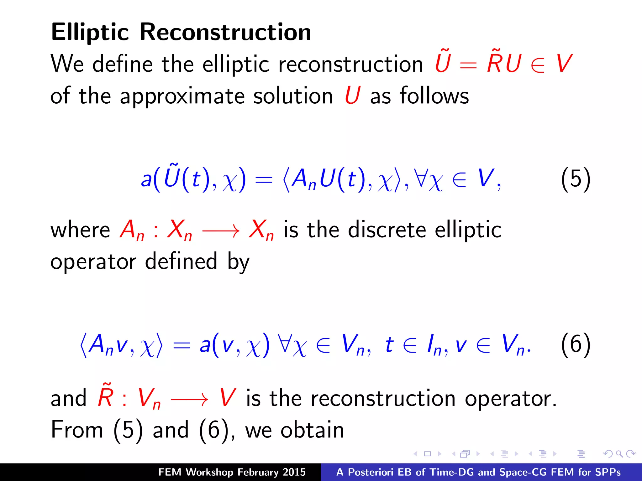
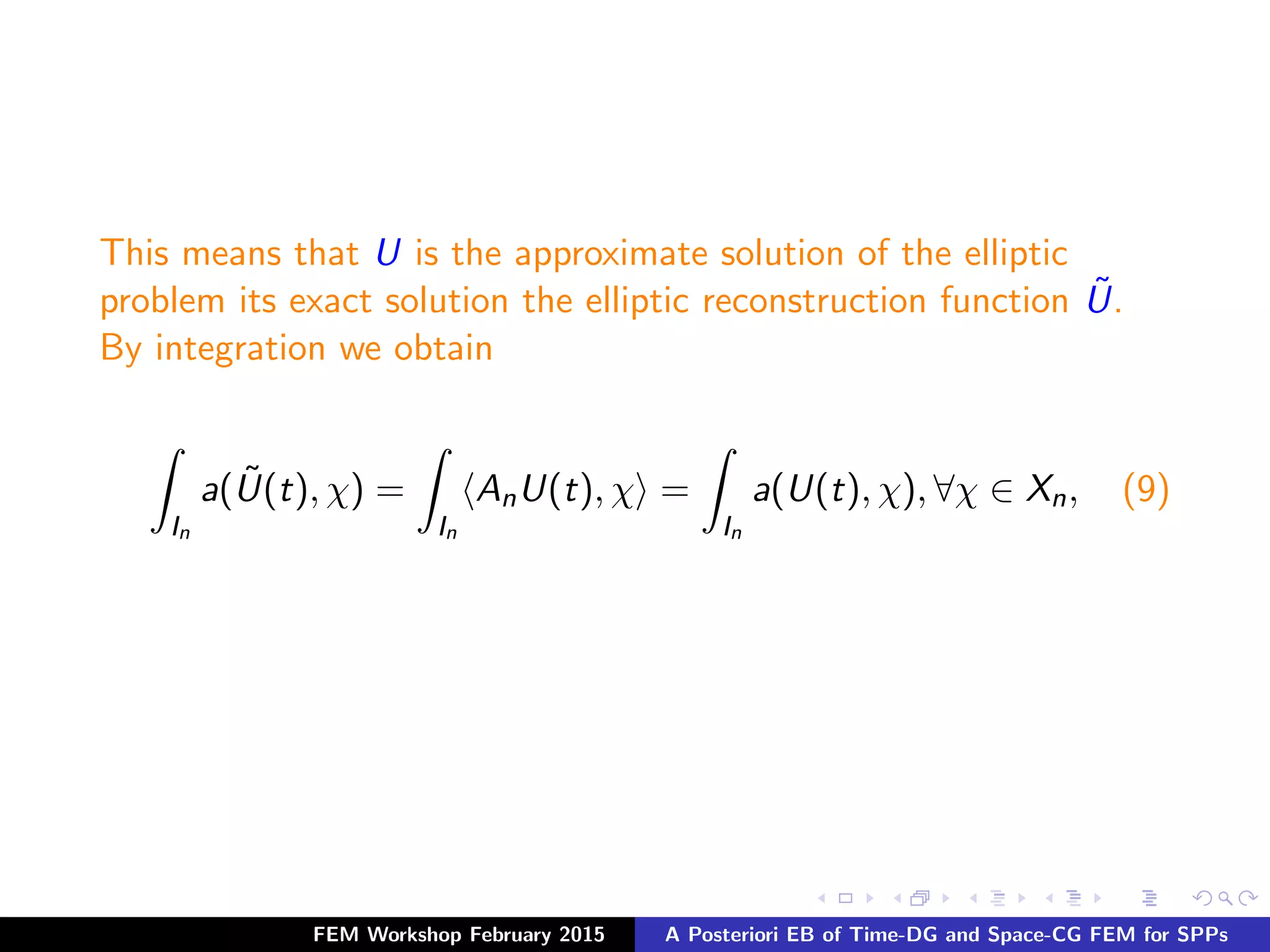
Time Reconstruction of the Elliptic Reconstruction
The time reconstruction function Û of the elliptic reconstruction ˜U
of the approximate solution U is defined by Û = ˆR ˜U where
ˆR : X(q) −→ X(q + 1) is the time reconstruction operator such
that Û|In ∈ Pqn+1 (In; V ) and
In
Û , v dt =
In
˜U , v dt + [ ˜U]n−1, v+
n−1 , ∀v ∈ X, (11)
Û+
0 = P1u0
Û+
n−1 = ˜U−
n−1, n > 0. (12)

Lemma 1(Continuity of the Time Reconstruction)
The time reconstruction deﬁned in (11-12) is well deﬁned and
globally continuous.

Theorem 2 (A posteriori Time Reconstruction
Error Bound)[SW10]
The following error estimate holds
ˆU − U L2(In;V ) = C2.6,kn,qn
[U]n−1 V + U−
n−1 − PnU−
n−1 V ,
(13)
where
C2.6,kn,qn
:=
k(q + 1)
(2q + 1)(2q + 3)
1/2
. (14)

Error Analysis and the Derivation of the Error
representation Formula
We can decompose the error in the following
ways[MLW]
e = u − U = (u − ˆU) + ( ˆU − U) = ˆρ + ˆ, (15)
and
e = u − U = (u − ˜U) + ( ˜U − U) = ˜ρ + ˜, (16)
noting that
e = u − U = ˆρ + ˆ = ˜ρ + ˜. (17)

We derive the a posteriori error bound for the error e by bounding
ˆρ and ˜ρ in terms of ˆ and ˜ which their a posteriori error bounds
are known and computable by Theorem 1 and Theorem 2.
The error representation formula for ˆρ and ˜ρ is
In
ˆρ , v + ˜ , v + a(˜ρ, v) dt − [U]n−1, v+
n−1
=
In
f (u) − Pnf (U), v dt, ∀v ∈ Xn. (18)

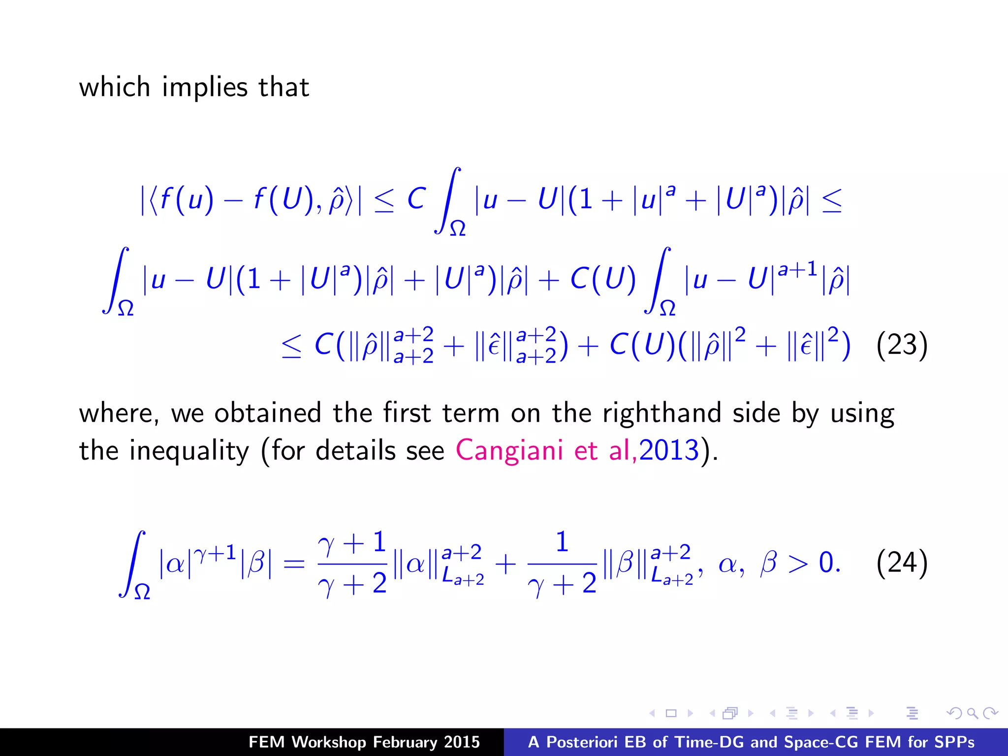
Testing (18) by v = ˆρ and by using continuity of the bilinear form
we obtain
In
ˆρ , ˆρ + ˜ , ˆρ + a(˜ρ, ˆρ) dt − [U]n−1, ˆρn−1
=
In
f (u) − Pnf (U), ˆρ dt, (19)
Now, we consider to bound the nonlinear term in the right hand
side of (19) which we decompose in the following way
f (u) − Pnf (U), ˆρ = f (u) − f (U) + f (U) − Pnf (U), ˆρ
= f (u) − f (U), ˆρ + f (U) − Pnf (U), ˆρ , (20)

The function f is locally Lipschitz continuous and satisﬁes the
following growth condition
|f (v) − f (w)| ≤ C|v − w|(1 + |v| + |w|)a
, 0 ≤ a < 2. (21)
where |.| is the Euclidean distance.
Now we need to bound this term by using the growth condition
(21),
Ω
|f (u) − f (U)||ˆρ| ≤ C
Ω
|u − U|(1 + |u|a
+ |U|a
)|ˆρ|. (22)

which implies that
| f (u) − f (U), ˆρ | ≤ C
Ω
|u − U|(1 + |u|a
+ |U|a
)|ˆρ| ≤
Ω
|u − U|(1 + |U|a
)|ˆρ| + |U|a
)|ˆρ| + C(U)
Ω
|u − U|a+1
|ˆρ|
≤ C( ˆρ a+2
a+2 + ˆ a+2
a+2) + C(U)( ˆρ 2
+ ˆ 2
) (23)
where, we obtained the ﬁrst term on the righthand side by using
the inequality (for details see Cangiani et al,2013).
Ω
|α|γ+1
|β| =
γ + 1
γ + 2
α a+2
La+2
+
1
γ + 2
β a+2
La+2
, α, β > 0. (24)

By using H¨older, Poincare and Sobolev inequalities inequality, we
have
ˆρ a+2
a+2 ≤ CS ˆρ a
ˆρ 2
V , (25)
and by the same way, we have
ˆ a+2
a+2 ≤ CS ˆ a
ˆ 2
V , (26)

Finally, we have
Ω
|f (u) − f (U)||ˆρ| ≤ C( ˆ a
ˆ 2
V + ˆρ a
ˆρ 2
V ) + C(U)( ˆρ 2
+ ˆ 2
),
(27)

After some mathematical manipulations and technicalities, we have
1
2
ˆρm
2
+
1
2
ˆρ 2
L2(Im;L2) +
C3
2
˜ρ 2
L2(Im;V ) +
1
2
ˆρ 2
L2(Im;V ) ≤
ˆρ0
2
+
1
2
m
n=1
[U]n−1
2
−
1
2
˜ 2
L2(Im;L2) +
C3
m
n=1 In
ˆ a
ˆ 2
V + C3
m
n=1 In
ˆρ a
ˆρ 2
V
+C5 ˆρ 2
L2(Im;L2) + C4 ˆ 2
L2(Im;L2) +
1
2
f (U) − Pnf (U) 2
L2(Im;L2),(28)

Now for simplicity let
δ2
= ˆρ0
2
+
1
2
m
n=1
[U]n−1
2
−
1
2
˜ 2
L2(Im;L2) + C3
m
n=1 In
ˆ a
ˆ 2
V
+C4 ˆ 2
L2(Im;L2) +
1
2
f (U) − Pnf (U) 2
L2(Im;L2),(29)
and by substituting δ2 in (28) we get
1
2
ˆρm
2
+
1
2
ˆρ 2
L2(Im;L2) +
C3
2
˜ρ 2
L2(Im;V ) +
1
2
ˆρ 2
L2(Im;V )
≤ δ2
+ C3
m
n=1 In
ˆρ a
ˆρ 2
V + C5 ˆρ 2
L2(Im;L2), (30)

implies that
1
2
ˆρm
2
+
1
2
ˆρ 2
L2(Im;L2) +
C3
2
˜ρ 2
L2(Im;V ) +
1
2
ˆρ 2
L2(Im;V )
≤ δ2
+ C3
m
n=1 In
sup
t∈In
ˆρ a
ˆρ 2
V + C5 ˆρ 2
L2(Im;L2) ≤
δ2
+ C3
m
n=1
sup
t∈In
ˆρ a
+
In
ˆρ 2
V
a+2
2
+ C5 ˆρ 2
L2(Im;L2), (31)

To bound the last term, we assume that kmax is the maximum time
stepsize be small enough such that kn ≤ kmax, ∀n and let δ be such
that
δ ≤
1
Ca
3 (4eC5T )
a+2
2a
=⇒ C3 4δ2
eC5T
a+2
2
≤ δ2
.
Now, consider the set
I = {t ∈ Im : sup
t∈Im
ˆρ 2
+
In
ˆρ 2
V ≤ 4δ2
eC5tm
}.

The set I is not empty and due to the continuity of the lefthand
side it is closed. Let t∗ = max I such that t∗ ≤ T and for t ≤ t∗,
we have
1
2
ˆρm
2
+
1
2
ˆρ 2
L2(Im;L2) +
C3
2
˜ρ 2
L2(Im;V ) +
1
2
ˆρ 2
L2(Im;V )
≤ 2δ2
+ C5 ˆρ 2
L2(Im;L2). (32)

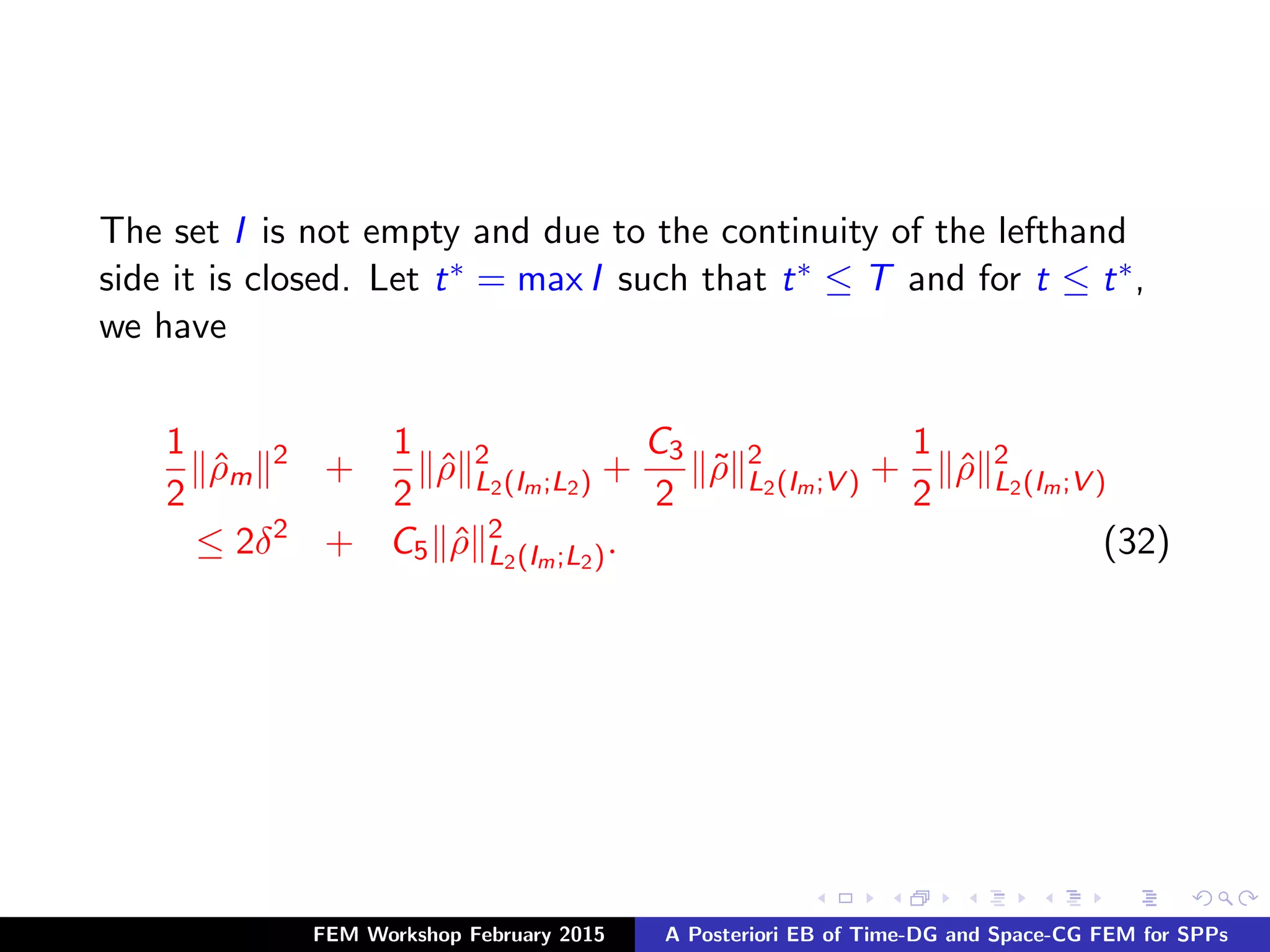
By using Gronwall’s inequality, we obtain
ˆρm
2
+ C3 ˜ρ(t∗
) 2
L2(Im;V ) + C6 ˆρ(t∗
) 2
L2(Im;V ) ≤ 4δ2
e2C7tm
. (33)
By choosing t = t∗, we have a contradiction to the assumption
that t < t∗ since the left hand side of (33) is continuous, therefore
we deduce that I = [0, tm].
Finally,
ˆρm
2
+ C3 ˜ρ 2
L2(Im;V ) + C6 ˆρ 2
L2(Im;V ) ≤ 4δ2
eC7tm
. (34)

Thank You
for Your Attention!

A Posteriori Error Analysis Presentation

Recommended

Recommended

More Related Content

What's hot

What's hot (20)

Similar to A Posteriori Error Analysis Presentation

Similar to A Posteriori Error Analysis Presentation (20)

More from Mohammad Sabawi Lecturer at Mathematics Department/College of Educations for Women/Tikrit University

More from Mohammad Sabawi Lecturer at Mathematics Department/College of Educations for Women/Tikrit University (7)

Recently uploaded

Recently uploaded (20)

A Posteriori Error Analysis Presentation