2020年5月7日 計算科学技術特論B
44
DGEMM tuned forthe K computer was also used for the
LINPACK benchmark program.
5.2 Scalability
We measured the computation time for the SCF iterations with
communications for the parallel tasks in orbitals, however, was
actually restricted to a relatively small number of compute nodes,
and therefore, the wall clock time for global communications of
the parallel tasks in orbitals was small. This means we succeeded
in decreasing time for global communication by the combination
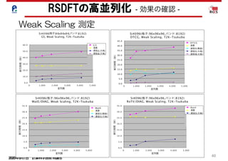
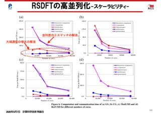
Figure 6. Computation and communication time of (a) GS, (b) CG, (c) MatE/SD and (d)
RotV/SD for different numbers of cores.
0.0
40.0
80.0
120.0
160.0
0 20000 40000 60000 80000
TimeperCG(sec.)
Number of cores
theoretical computation
computation
adjacent/space
global/space
global/orbital
0.0
100.0
200.0
300.0
400.0
0 20,000 40,000 60,000 80,000
TimeperGS(sec.)
Number of cores
theoretical computation
computation
global/space
global/orbital
wait/orbital
0.0
50.0
100.0
150.0
200.0
0 20,000 40,000 60,000 80,000
TimeperMatE/SD(sec.)
Number of cores
theoretical computation
computation
adjacent/space
global/space
global/orbital
0.0
100.0
200.0
300.0
0 20,000 40,000 60,000 80,000
TimeperRotV/SD(sec.)
Number of cores
theoretical computation
computation
adjacent/space
global/space
global/orbital
(d)(c)
(a) (b)
time as a result of keeping the block data on the L1 cache
manually decreased by 12% compared with the computation time
for the usual data replacement operations of the L1 cache. This
DGEMM tuned for the K computer was also used for the
LINPACK benchmark program.
5.2 Scalability
We measured the computation time for the SCF iterations with
hand, the global communication time for the parallel tasks in
orbitals was supposed to increase as the number of parallel tasks
in orbitals increased. The number of MPI processes requiring
communications for the parallel tasks in orbitals, however, was
actually restricted to a relatively small number of compute nodes,
and therefore, the wall clock time for global communications of
the parallel tasks in orbitals was small. This means we succeeded
in decreasing time for global communication by the combination
Figure 6. Computation and communication time of (a) GS, (b) CG, (c) MatE/SD and (d)
RotV/SD for different numbers of cores.
0.0
40.0
80.0
120.0
160.0
0 20000 40000 60000 80000
TimeperCG(sec.)
Number of cores
theoretical computation
computation
adjacent/space
global/space
global/orbital
0.0
100.0
200.0
300.0
400.0
0 20,000 40,000 60,000 80,000
TimeperGS(sec.)
Number of cores
theoretical computation
computation
global/space
global/orbital
wait/orbital
0.0
50.0
100.0
150.0
200.0
0 20,000 40,000 60,000 80,000
TimeperMatE/SD(sec.)
Number of cores
theoretical computation
computation
adjacent/space
global/space
global/orbital
0.0
100.0
200.0
300.0
0 20,000 40,000 60,000 80,000TimeperRotV/SD(sec.)
Number of cores
theoretical computation
computation
adjacent/space
global/space
global/orbital
(d)(c)
(a) (b)
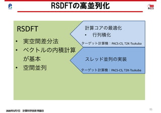
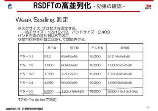
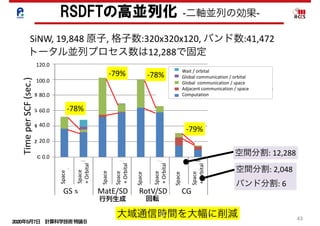
RSDFTの高並列化-スケーラビリティ-
並列度のミスマッチの解消
大域通信の増大の解消
45.
2020年5月7日 計算科学技術特論B
45
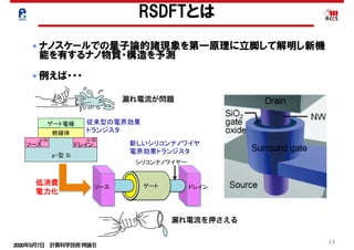
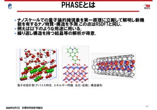
confinement becomes prominent.The quantum effects,
which depend on the crystallographic directions of the nano-
wire axes and on the cross-sectional shapes of the nanowires,
result in substantial modifications to the energy-band
structures and the transport characteristics of SiNW FETs.
However, knowledge of the effect of the structural mor-
phology on the energy bands of SiNWs is lacking. In addi-
tion, actual nanowires have side-wall roughness. The
effects of such imperfections on the energy bands are
Table 2. Distribution of computational costs for an iteration of the SCF calculation of the modified code.
Procedure block
Execution
time (s)
Computation
time (s)
Communication time (s)
Performance
(PFLOPS/%)Adjacent/grids Global/grids Global/orbitals Wait/orbitals
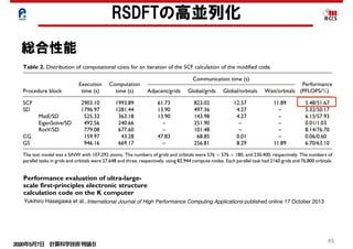
SCF 2903.10 1993.89 61.73 823.02 12.57 11.89 5.48/51.67
SD 1796.97 1281.44 13.90 497.36 4.27 – 5.32/50.17
MatE/SD 525.33 363.18 13.90 143.98 4.27 – 6.15/57.93
EigenSolve/SD 492.56 240.66 – 251.90 – – 0.01/1.03
RotV/SD 779.08 677.60 – 101.48 – – 8.14/76.70
CG 159.97 43.28 47.83 68.85 0.01 – 0.06/0.60
GS 946.16 669.17 – 256.81 8.29 11.89 6.70/63.10
The test model was a SiNW with 107,292 atoms. The numbers of grids and orbitals were 576 Â 576 Â 180, and 230,400, respectively. The numbers of
parallel tasks in grids and orbitals were 27,648 and three, respectively, using 82,944 compute nodes. Each parallel task had 2160 grids and 76,800 orbitals.
Hasegawa et al. 13
Article
Performance evaluation of ultra-large-
scale first-principles electronic structure
calculation code on the K computer
Yukihiro Hasegawa1
, Jun-Ichi Iwata2
, Miwako Tsuji1
,
Daisuke Takahashi3
, Atsushi Oshiyama2
, Kazuo Minami1
,
Taisuke Boku3
, Hikaru Inoue4
, Yoshito Kitazawa5
,
Ikuo Miyoshi6
and Mitsuo Yokokawa7,1
Abstract
The International Journal of High
Performance Computing Applications
1–21
ª The Author(s) 2013
Reprints and permissions:
sagepub.co.uk/journalsPermissions.nav
DOI: 10.1177/1094342013508163
hpc.sagepub.com
Yukihiro Hasegawa et al.,
http://hpc.sagepub.com/
Computing Applications
International Journal of High Performance
http://hpc.sagepub.com/content/early/2013/10/16/1094342013508163
The online version of this article can be found at:
DOI: 10.1177/1094342013508163
published online 17 October 2013International Journal of High Performance Computing Applications
Hikaru Inoue, Yoshito Kitazawa, Ikuo Miyoshi and Mitsuo Yokokawa
Yukihiro Hasegawa, Jun-Ichi Iwata, Miwako Tsuji, Daisuke Takahashi, Atsushi Oshiyama, Kazuo Minami, Taisuke Boku,
K computer
Performance evaluation of ultra-largescale first-principles electronic structure calculation code on the
Published by:
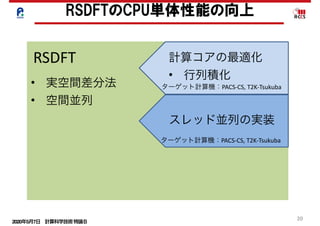
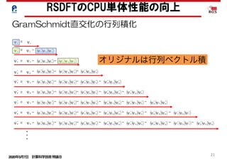
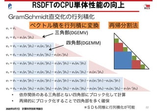
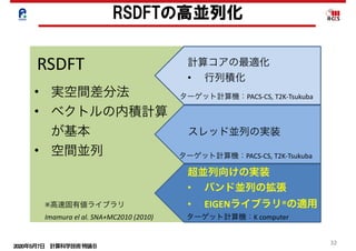
RSDFTの高並列化
総合性能
2020年5月7日 計算科学技術特論B
63
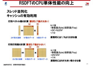
スレッド並列化
キャッシュの有効利用-行列積化
0
50
100
150
200
250
300
orinigal original+DGEMM 22axis+1threads22axis+8threads
[s]
Algorithm
Gram/Schmidt3orthonormalization
other
M× M
M× V
「京」
PHASEの高並列化・高性能化の結果
行列積
行列ベクトル積
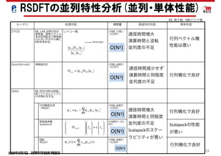
第 4 章 高並列性能最適化技術の研究
三角の処理部分は行列ベクトル積計算が残っており、細字の 2 サブルーチンがこ
する。行列ベクトル積に比べ行列行列積は、8 から 15 倍程度性能が向上している
る。区間 5 全体で見ても実効効率 28%を達成した。
Table 4.11: PHASE の行列行列積化の結果
サブルーチン
時間
(sec)
比率
(%)
演算効率
(%)
区間 5 512.7 100.0 28.23
m ES F transpose r 105.3 20.5 0
m ES W transpose r 15.7 3.1 0
WSW t 15.2 3.0 0.036
normalize bp and psi t 0.9 0.2 3.25
W1SW2 t r 49.2 9.6 5.46
modify bp and psi t r 50.8 9.9 4.45
W1SW2 t r block 162.0 31.6 41.89
modify bp and psi t r block 96.2 18.8 74.65
m ES W transpose back r 14.1 2.8 0
m ES F transpose back r 1.3 0.3 0
「京」
![2020年5月7日 計算科学技術特論B
52
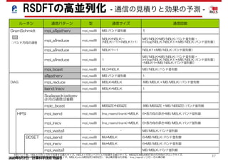
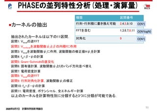
■行列積カーネル
PHASEの処理ブロック:区間2を例に示す.
低並列でストロングスケールで測定.
HfSiO2 384原子アモルファス系を測定
! BLAS Level3
!
BLAS Level3 ( 2)
(
0
2
4
6
8
10
12
14
16 32 64
[s]
AS Level3
LAS Level3 ( 2)
(
0
2
4
6
8
10
12
14
16 32 64 128
[s]
original:0calc.
23axis:0calc.
23axis:0comm.
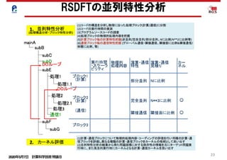
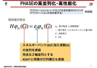
区間2: Vnonlocalを波動関数ψiとβの内積fに作用
区間4: fijt=β・ψの計算
区間10: fijt=β・ψの計算
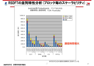
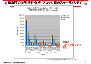
PHASEの並列特性分析(ブロック毎のスケーラビリティ)
すでにこの並列度でスケールしていない.
原因は非並列部の残存.
区間4,10も同様](https://image.slidesharecdn.com/200507materialminami-200428004429/85/slide-52-320.jpg)
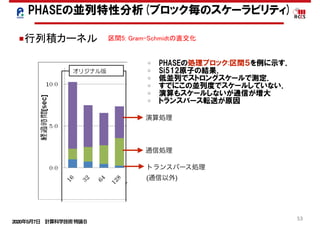
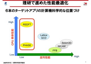
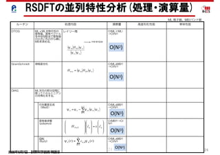
 1.00 1.05 1.06 1.08
高速化率 [-](固有値
計算含まず) 1.00 1.81 3.03 4.60
PHASEの並列特性分析(ブロック毎のスケーラビリティ)](https://image.slidesharecdn.com/200507materialminami-200428004429/85/slide-55-320.jpg)
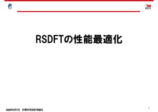
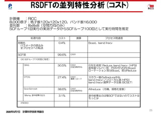
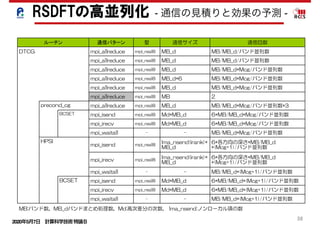
![2020年5月7日 計算科学技術特論B
63
スレッド並列化
キャッシュの有効利用-行列積化
0
50
100
150
200
250
300
orinigal original+DGEMM 22axis+1threads 22axis+8threads
[s]
Algorithm
Gram/Schmidt3orthonormalization
other
M× M
M× V
「京」
PHASEの高並列化・高性能化の結果
行列積
行列ベクトル積
第 4 章 高並列性能最適化技術の研究
三角の処理部分は行列ベクトル積計算が残っており、細字の 2 サブルーチンがこ
する。行列ベクトル積に比べ行列行列積は、8 から 15 倍程度性能が向上している
る。区間 5 全体で見ても実効効率 28%を達成した。
Table 4.11: PHASE の行列行列積化の結果
サブルーチン
時間
(sec)
比率
(%)
演算効率
(%)
区間 5 512.7 100.0 28.23
m ES F transpose r 105.3 20.5 0
m ES W transpose r 15.7 3.1 0
WSW t 15.2 3.0 0.036
normalize bp and psi t 0.9 0.2 3.25
W1SW2 t r 49.2 9.6 5.46
modify bp and psi t r 50.8 9.9 4.45
W1SW2 t r block 162.0 31.6 41.89
modify bp and psi t r block 96.2 18.8 74.65
m ES W transpose back r 14.1 2.8 0
m ES F transpose back r 1.3 0.3 0
「京」](https://image.slidesharecdn.com/200507materialminami-200428004429/85/slide-63-320.jpg)
![2020年5月7日 計算科学技術特論B
64
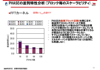
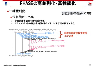
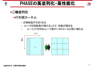
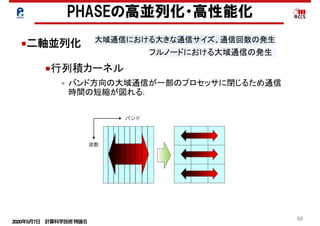
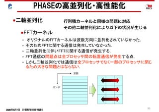
■二軸並列化
• 行列積化されたカーネルに(区間2)ついての結果.
• HfSiO2 384原子アモルファス系のデータ.
• 大幅な性能向上を達成.
PHASEの高並列化・高性能化の結果
■行列積カーネル
0.0
2.0
4.0
6.0
8.0
10.0
12.0
14.0
16.0
18.0
20.0
16 32 64 128
プロセス数
経過時間[sec]
0.0
2.0
4.0
6.0
8.0
10.0
12.0
14.0
16.0
18.0
20.0
プロセス数
経過時間[sec]
通信部 主要演算ループ
0
2
4
6
8
10
12
14
16 32 64 128
[s]
プロセス数
original:0calc.
23axis:0calc.
23axis:0comm.
FX1
「京」](https://image.slidesharecdn.com/200507materialminami-200428004429/85/slide-64-320.jpg)
![2020年5月7日 計算科学技術特論B
65
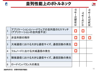
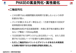
■二軸並列化
• FFTを含むカーネルに(区間8)ついての結果.
• HfSiO2 384原子アモルファス系のデータ.
• 性能向上を達成.
PHASEの高並列化・高性能化の結果
■FFTカーネル
プロセス数
0.0
10.0
20.0
30.0
40.0
50.0
16 32 64 128
経過時間[sec]
0.0
10.0
20.0
30.0
40.0
50.0
プロセス数
経過時間[sec]
0
2
4
6
8
10
12
14
16
18
16 32 64 128
[s]
プロセス数
original:0other
original:0DGEMM
original:0FFT
2:axis:0other
2:axis:0comm.
2:axis:0DGEMM
2:axis:0FFT
FX1
「京」](https://image.slidesharecdn.com/200507materialminami-200428004429/85/slide-65-320.jpg)
![2020年5月7日 計算科学技術特論B
66
■Scalapack分割数の固定
• 対角化はエネルギーバンド数の元を持つ行列が対象
• 行列の大きさに比べて分割数が多すぎる
• 分割数を16 16=256に固定
PHASEの高並列化・高性能化の結果
■対角化カーネル
区間9の実行時間と分割数の関係.
0
100
200
300
400
500
600
700
0
20
40
60
80
100
0 10 20 30 40
[s][s]
分割数
HfSiO4_3072
HfSiO4_6144
0
50
100
150
200
250
16x32 16x64 16x96 16x128 16x160
[s]
プロセス数(バンド×波数)
ScaLAPACK
FFT
BLAS
「京」「京」](https://image.slidesharecdn.com/200507materialminami-200428004429/85/slide-66-320.jpg)
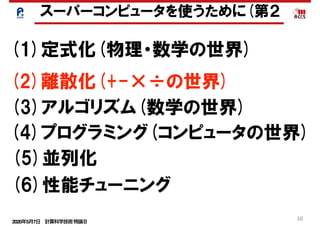
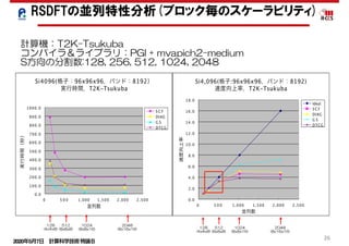
![2020年5月7日 計算科学技術特論B
67
PHASEの高並列化・高性能化の結果
総合性能
0
200
400
600
800
1000
1200
1400
48 96 192 384 768 1536 3072 6114 12288
Time%[s]
Process
DGEMM
FFT
ScaLAPACK
■ 「京」 2048並列にて,アモルファス1536原子
計算の性能.ピーク性能比20.1%.
e 4.13 に HfSiO2、1536 原子アモルファス系を用いて、「京」コンピュータ、2048
実測した実行時間と実行効率を示した。BLAS 化した箇所は 40%以上の実行効率
し、SCF ループ全体を通じて 20%を越える実行効率を達成できた。Fig. 4.25 は同
各並列数でのカーネル種別ごとの実行時間の内訳である。HfSiO2、1536 原子の場
00 並列程度まで並列性能が保たれるのを確認した。この計算ではすでに並列数が原
上回っており、今までの並列手法では分割粒度が細かく計算不可能な問題である。
26 は、SiC3800 原子系を 48 並列から 12288 並列まで測定した結果を示す。原子数
るかに大きい並列数までスケールが確保できることが示されている。
able 4.13: PHASE の 1536 原子アモルファス系の 2048 並列での性能 (「京」)
区間名
実行時間
(sec)
浮動小数点演算
ピーク比
SCF 39.79 20.11%
区間 1(FFT) 0.02 2.19%
区間 2(BLAS) 6.89 53.53%
区間 3(FFT) 3.99 3.56%
区間 4(BLAS) 1.88 64.76%
区間 5(BLAS, 通信) 2.53 17.32%
区間 6(FFT) 1.24 5.15%
区間 8(FFT,BLAS) 4.16 16.56%
区間 9(BLAS,ScaLAPACK) 12.31 3.88%
区間 10(BLAS) 1.89 64.30%
区間 11(FFT) 5.05 4.78%
得られれ
は 30%程
と予測で
8 並列で
. BLAS
し,SCF
率を達成
種別毎の
子の場合
確認した.
っており,
計算不可
算できた
LAS を導
T を含む
下の効率
リケーシ
画期的と
どの全体通信を含む通信アルゴリズムの性能低下
が危惧されていたが,並列軸の追加により,通信を
グループ化でき,超並列にもある程度対応可能であ
ることが示唆された.FFT に関しては,今後「京」
では,多次元並列版 FFT が整備されるなど,更な
る高速化が期待される.更に現在 FFT を行うため
にパッキングなどの前処理を行っているが,この箇
所のデータを連続化することで,更に並列効率の向
上が見込まれる.
対角化については,汎用ライブラリでは,それほ
ど並列性能が見込まれないが,必要とする計算が全
空間での対角化ではなく,部分空間という比較的小
規模な対角化であるため,1,000 並列程度とある程
度並列性能が保証されていれば,全体の計算時間へ
の影響は低く抑えられると考えている.今後,高並
列版対角化ライブラリを導入することで,より高並
列にも対応可能である.
本アプリケーションは「京」共用開始時に,SCF
収束回数を考慮しても,理論上は 100,000 原子程度
の電子状態計算が日単位で達成できる見込みであ
る.しかし様々なデバイス特性を調べるために,分
子動力学計算や反応中間体の計算などを実施する
場合,収束時間を短くしなければならないという要
ーク比
各カ
100.0
120.0
140.0
160.0
[s]
ScaLAPACK
FFT
BLAS
■ SiC 3800原子系を「京」48並列から12288並
列まで原子数よりはるかに多い並列度まで
スケールすることを確認.
■ 「京」 3072並列にてSiC 4096原子計算にて,構
造緩和 (263MD, 2days).
■ 「京」82944並列にてSiC 20440原子計算のMSD
ソルバー効率 20.2 % (2.1 PFLOPS)達成.](https://image.slidesharecdn.com/200507materialminami-200428004429/85/slide-67-320.jpg)