Software Reliability
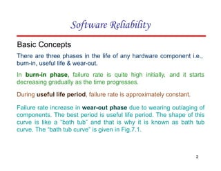
Basic Concepts
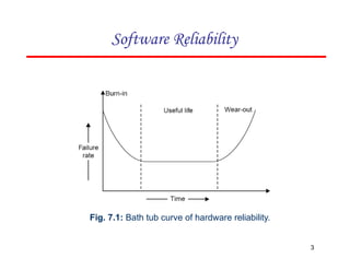
Thereare three phases in the life of any hardware component i.e.,
burn-in, useful life & wear-out.
In burn-in phase, failure rate is quite high initially, and it starts
decreasing gradually as the time progresses.
During useful life period, failure rate is approximately constant.
Failure rate increase in wear-out phase due to wearing out/aging of
components. The best period is useful life period. The shape of this
curve is like a “bath tub” and that is why it is known as bath tub
curve. The “bath tub curve” is given in Fig.7.1.
2
3.
Fig. 7.1: Bathtub curve of hardware reliability.
Software Reliability
3
4.
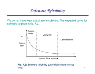
Fig. 7.2: Softwarereliability curve (failure rate versus
time)
Software Reliability
We do not have wear out phase in software. The expected curve for
software is given in fig. 7.2.
4
5.
Software may beretired only if it becomes obsolete. Some of
contributing factors are given below:
✓ change in environment
✓ change in infrastructure/technology
✓ major change in requirements
✓ increase in complexity
✓ extremely difficult to maintain
✓ deterioration in structure of the code
✓ slow execution speed
✓ poor graphical user interfaces
Software Reliability
5
6.
Software Reliability
What isSoftware Reliability?
“Software reliability means operational reliability. Who cares how
many bugs are in the program?
As per IEEE standard: “Software reliability is defined as the ability of
a system or component to perform its required functions under
stated conditions for a specified period of time”.
6
7.
Software reliability isalso defined as the probability that a software
system fulfills its assigned task in a given environment for a
predefined number of input cases, assuming that the hardware and
the inputs are free of error.
“It is the probability of a failure free operation of a program for a
specified time in a specified environment”.
7
Software Reliability
8.
▪ Failures andFaults
A fault is the defect in the program that, when executed under
particular conditions, causes a failure.
The execution time for a program is the time that is actually spent by
a processor in executing the instructions of that program. The
second kind of time is calendar time. It is the familiar time that we
normally experience.
8
Software Reliability
9.
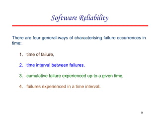
There are fourgeneral ways of characterising failure occurrences in
time:
1. time of failure,
2. time interval between failures,
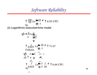
3. cumulative failure experienced up to a given time,
4. failures experienced in a time interval.
9
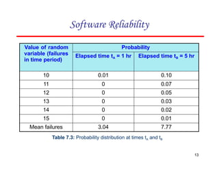
Software Reliability
12
Value of random
variable(failures
in time period)
Probability
Elapsed time tA = 1 hr Elapsed time tB = 5 hr
0 0.10 0.01
1 0.18 0.02
2 0.22 0.03
3 0.16 0.04
4 0.11 0.05
5 0.08 0.07
6 0.05 0.09
7 0.04 0.12
8 0.03 0.16
9 0.02 0.13
Table 7.3: Probability distribution at times tA and tB
Software Reliability
13.
Value of random
variable(failures
in time period)
Probability
Elapsed time tA = 1 hr Elapsed time tB = 5 hr
10 0.01 0.10
11 0 0.07
12 0 0.05
13 0 0.03
14 0 0.02
15 0 0.01
Mean failures 3.04 7.77
13
Table 7.3: Probability distribution at times tA and tB
Software Reliability
14.
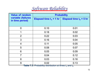
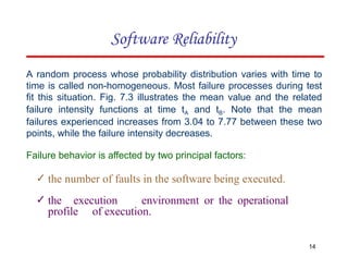
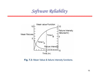
A random processwhose probability distribution varies with time to
time is called non-homogeneous. Most failure processes during test
fit this situation. Fig. 7.3 illustrates the mean value and the related
failure intensity functions at time tA and tB. Note that the mean
failures experienced increases from 3.04 to 7.77 between these two
points, while the failure intensity decreases.
Failure behavior is affected by two principal factors:
✓ the number of faults in the software being executed.
✓ the execution environment or the operational
profile of execution.
14
Software Reliability
Environment
The environment isdescribed by the operational profile. The
proportion of runs of various types may vary, depending on the
functional environment. Examples of a run type might be:
1. a particular transaction in an airline reservation system or a
business data processing system,
2. a specific cycle in a closed loop control system
(for example, in a chemical process industry),
3. a particular service performed by an operating system for a
user.
16
Software Reliability
17.
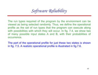
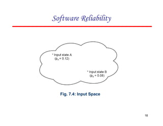
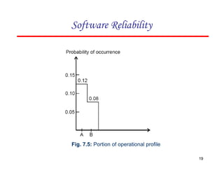
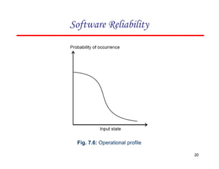
The run typesrequired of the program by the environment can be
viewed as being selected randomly. Thus, we define the operational
profile as the set of run types that the program can execute along
with possibilities with which they will occur. In fig. 7.4, we show two
of many possible input states A and B, with their probabilities of
occurrence.
The part of the operational profile for just these two states is shown
in fig. 7.5. A realistic operational profile is illustrated in fig.7.6.
17
Software Reliability
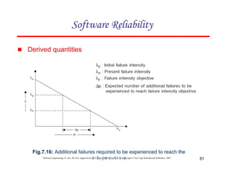
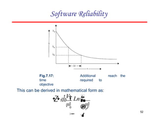
Software Reliability
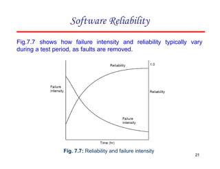
Fig. 7.7:Reliability and failure intensity
Fig.7.7 shows how failure intensity and reliability typically vary
during a test period, as faults are removed.
21
22.
Uses of ReliabilityStudies
There are at least four other ways in which software reliability
measures can be of great value to the software engineer, manager
or user.
1. you can use software reliability measures to evaluate software
engineering technology quantitatively.
22
2. software
evaluating
project.
reliability measures offer you the
possibility of development status
during the test phasesof
a
Software Reliability
23.
3. one canuse software reliability measures to monitor the
operational performance of software and to control new features
added and design changes made to the software.
4. a quantitative understanding of software quality and the various
factors influencing it and affected by it enriches into the
software product and the software development process.
23
Software Reliability
24.
Software Quality
Different peopleunderstand different meanings of quality like:
❖ conformance to requirements
❖ fitness for the purpose
❖ level of satisfaction
24
Software Reliability
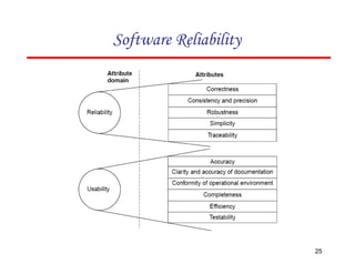
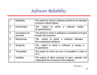
Software Reliability
1 ReliabilityThe extent to which a software performs its intended
functions without failure.
2 Correctness The extent to which a software meets
its specifications.
3 Consistency &
precision
The extent to which a software is consistent and give
results with precision.
4 Robustness The extent to which a software tolerates
the unexpected problems.
5 Simplicity The extent to which a software is simple in
its operations.
6 Traceability The extent to which an error is traceable in order to
fix it.
7 Usability The extent of effort required to learn, operate and
understand the functions of the software
27
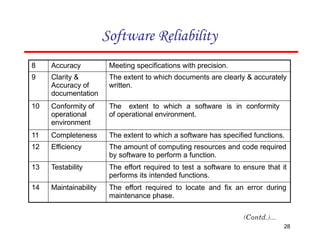
28.
Software Reliability
8 AccuracyMeeting specifications with precision.
9 Clarity &
Accuracy of
documentation
The extent to which documents are clearly & accurately
written.
10 Conformity of
operational
environment
The extent to which a software is in conformity
of operational environment.
11 Completeness The extent to which a software has specified functions.
12 Efficiency The amount of computing resources and code required
by software to perform a function.
13 Testability The effort required to test a software to ensure that it
performs its intended functions.
14 Maintainability The effort required to locate and fix an error during
maintenance phase.
28
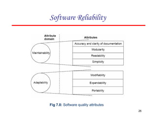
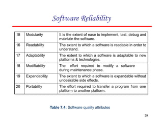
29.
Software Reliability
29
15 ModularityIt is the extent of ease to implement, test, debug and
maintain the software.
16 Readability The extent to which a software is readable in order to
understand.
17 Adaptability The extent to which a software is adaptable to new
platforms & technologies.
18 Modifiability The effort required to modify a software
during maintenance phase.
19 Expandability The extent to which a software is expandable without
undesirable side effects.
20 Portability The effort required to transfer a program from one
platform to another platform.
Table 7.4: Software quality attributes
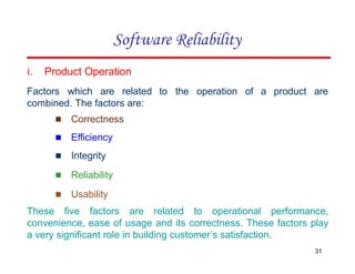
to the operationof a product are
31
combined. The factors are:
▪ Correctness
▪ Efficiency
▪ Integrity
▪ Reliability
▪ Usability
i. Product Operation
Factors which are related
These five factors are related to operational performance,
convenience, ease of usage and its correctness. These factors play
a very significant role in building customer’s satisfaction.
Software Reliability
32.
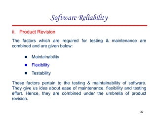
ii. Product Revision
Thefactors which are required for testing & maintenance are
combined and are given below:
▪ Maintainability
▪ Flexibility
▪ Testability
These factors pertain to the testing & maintainability of software.
They give us idea about ease of maintenance, flexibility and testing
effort. Hence, they are combined under the umbrella of product
revision.
32
Software Reliability
33.
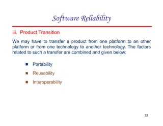
iii. Product Transition
Wemay have to transfer a product from one platform to an other
platform or from one technology to another technology. The factors
related to such a transfer are combined and given below:
▪ Portability
▪ Reusability
▪ Interoperability
33
Software Reliability
34.
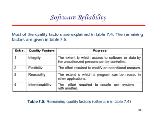
Most of thequality factors are explained in table 7.4. The remaining
factors are given in table 7.5.
34
Software Reliability
Sr.No. Quality Factors Purpose
1 Integrity The extent to which access to software or data by
the unauthorized persons can be controlled.
2 Flexibility The effort required to modify an operational program.
3 Reusability The extent to which a program can be reused in
other applications.
4 Interoperability The effort required to couple one system
with another.
Table 7.5: Remaining quality factors (other are in table 7.4)
Software Reliability
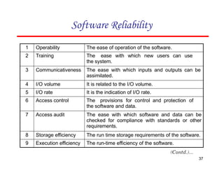
1 OperabilityThe ease of operation of the software.
2 Training The ease with which new users can use
the system.
3 Communicativeness The ease with which inputs and outputs can be
assimilated.
4 I/O volume It is related to the I/O volume.
5 I/O rate It is the indication of I/O rate.
6 Access control The provisions for control and protection of
the software and data.
7 Access audit The ease with which software and data can be
checked for compliance with standards or other
requirements.
8 Storage efficiency The run time storage requirements of the software.
9 Execution efficiency The run-time efficiency of the software.
37
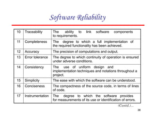
38.
Software Reliability
10 TraceabilityThe ability to link software components
to requirements.
11 Completeness The degree to which a full implementation of
the required functionality has been achieved.
12 Accuracy The precision of computations and output.
13 Error tolerance The degree to which continuity of operation is ensured
under adverse conditions.
14 Consistency The use of uniform design and
implementation techniques and notations throughout a
project.
15 Simplicity The ease with which the software can be understood.
16 Conciseness The compactness of the source code, in terms of lines
of code.
17 Instrumentation The degree to which the software provides
for measurements of its use or identification of errors.
38
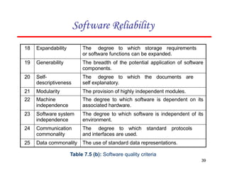
39.
Software Reliability
39
18 ExpandabilityThe degree to which storage requirements
or software functions can be expanded.
19 Generability The breadth of the potential application of software
components.
20 Self-
descriptiveness
The degree to which the documents are
self explanatory.
21 Modularity The provision of highly independent modules.
22 Machine
independence
The degree to which software is dependent on its
associated hardware.
23 Software system
independence
The degree to which software is independent of its
environment.
24 Communication
commonality
The degree to which standard protocols
and interfaces are used.
25 Data commonality The use of standard data representations.
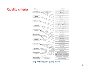
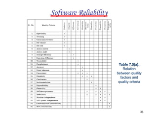
Table 7.5 (b): Software quality criteria
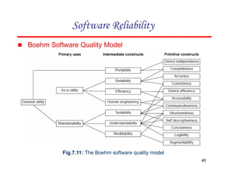
40.
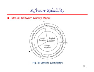
▪ Boehm SoftwareQuality Model
40
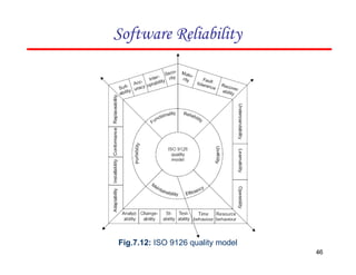
Fig.7.11: The Boehm software quality model
Software Reliability
Software Reliability
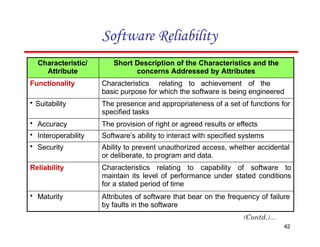
Characteristic/
Attribute
Short Descriptionof the Characteristics and the
concerns Addressed by Attributes
Functionality Characteristics relating to achievement of the
basic purpose for which the software is being engineered
• Suitability The presence and appropriateness of a set of functions for
specified tasks
• Accuracy The provision of right or agreed results or effects
• Interoperability Software’s ability to interact with specified systems
• Security Ability to prevent unauthorized access, whether accidental
or deliberate, to program and data.
Reliability Characteristics relating to capability of software to
maintain its level of performance under stated conditions
for a stated period of time
• Maturity Attributes of software that bear on the frequency of failure
by faults in the software
42
43.
Software Reliability
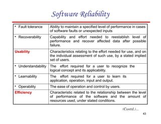
• Faulttolerance Ability to maintain a specified level of performance in cases
of software faults or unexpected inputs
• Recoverability Capability and effort needed to reestablish level of
performance and recover affected data after possible
failure.
Usability Characteristics relating to the effort needed for use, and on
the individual assessment of such use, by a stated implied
set of users.
• Understandability The effort required for a user to recognize the
logical concept and its applicability.
• Learnability The effort required for a user to learn its
application, operation, input and output.
• Operability The ease of operation and control by users.
Efficiency Characteristic related to the relationship between the level
of performance of the software and the amount of
resources used, under stated conditions.
43
44.
Software Reliability
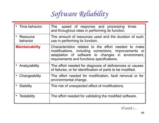
• Timebehavior The speed of response and processing times
and throughout rates in performing its function.
• Resource
behavior
The amount of resources used and the duration of such
use in performing its function.
Maintainability Characteristics related to the effort needed to make
modifications, including corrections, improvements or
adaptation of software to changes in environment,
requirements and functions specifications.
• Analyzability The effort needed for diagnosis of deficiencies or causes
of failures, or for identification of parts to be modified.
• Changeability The effort needed for modification, fault removal or for
environmental change.
• Stability The risk of unexpected effect of modifications.
• Testability The effort needed for validating the modified software.
44
45.
Software Reliability
45
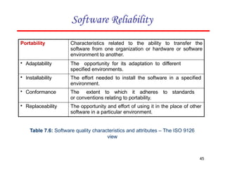
Portability Characteristicsrelated to the ability to transfer the
software from one organization or hardware or software
environment to another.
• Adaptability The opportunity for its adaptation to different
specified environments.
• Installability The effort needed to install the software in a specified
environment.
• Conformance The extent to which it adheres to standards
or conventions relating to portability.
• Replaceability The opportunity and effort of using it in the place of other
software in a particular environment.
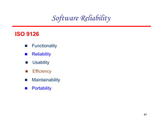
Table 7.6: Software quality characteristics and attributes – The ISO 9126
view
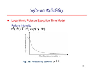
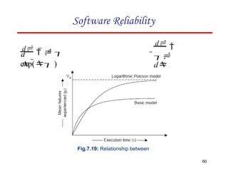
Software Reliability Models
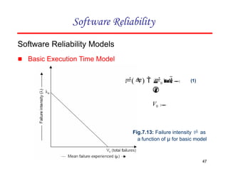
▪Basic Execution Time Model
47
() 0 1
V0
Fig.7.13: Failure intensity as
a function of µ for basic model
(1)
Software Reliability
48.
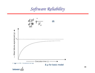
d V0
d
0
&µ for basic model
Fig.7.14: Relationship
between
(2)
48
Software Reliability
49.
49
0
0
d(
)V
(
)
1
d
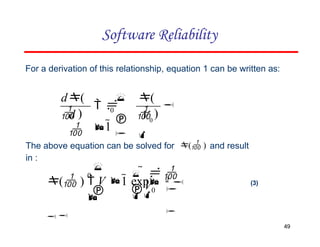
For a derivation of this relationship, equation 1 can be written as:
The above equation can be solved for ( ) and result
in :
0
0
V
( ) V 1 exp 0
(3)
Software Reliability
50.
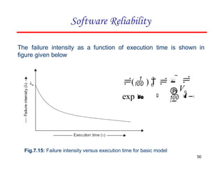
Fig.7.15: Failure intensityversus execution time for basic model
The failure intensity as a function of execution time is shown in
figure given below
0
50
0
V
( )
exp 0
Software Reliability
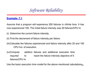
Example- 7.1
Assume thata program will experience 200 failures in infinite time. It has
now experienced 100. The initial failure intensity was 20 failures/CPU hr.
(i) Determine the current failure intensity.
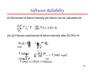
(ii) Find the decrement of failure intensity per failure.
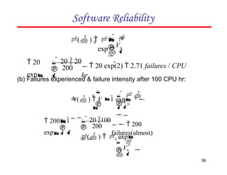
(iii)Calculate the failures experienced and failure intensity after 20 and 100
CPU hrs. of execution.
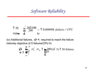
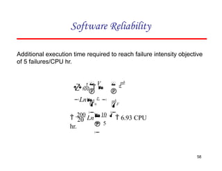
(iv)Compute addition failures and additional execution time
required to reach the failure intensity objective of 5
failures/CPU hr.
Use the basic execution time model for the above mentioned calculations.
Software Reliability
53
Example- 7.2
Assume thatthe initial failure intensity is 20 failures/CPU hr. The failure
intensity decay parameter is 0.02/failures. We have experienced 100
failures up to this time.
(i) Determine the current failure intensity.
(ii) Calculate the decrement of failure intensity per failure.
(iii)Find the failures experienced and failure intensity after 20 and 100 CPU
hrs. of execution.
(iv)Compute the additional failures and additional execution time required to
reach the failure intensity objective of 2 failures/CPU hr.
Use Logarithmic Poisson execution time model for the above mentioned
calculations.
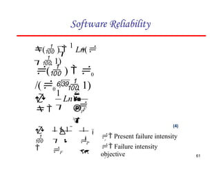
Software Reliability
62
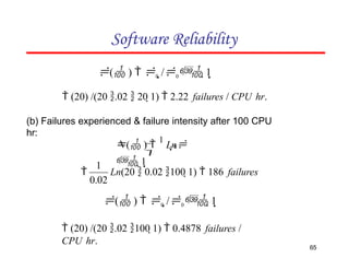
Example- 7.3
The followingparameters for basic and logarithmic Poisson models are
given:
(a) Determine the addition failures and additional execution time required to
reach the failure intensity objective of 5 failures/CPU hr. for both
models.
(b) Repeat this for an objective function of 0.5 failure/CPU hr. Assume that
we start with the initial failure intensity only.
Software Reliability
67
Basic execution time model Logarithmic Poisson
execution time model
10 failures/CPU hr
o
30 failures/CPU hr
o
V 100 failures
o
0.25 / failure
68.
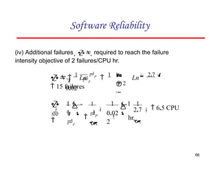
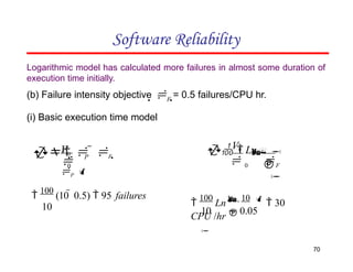
Solution
(a) (i) Basicexecution time model
Software Reliability
0
P F
V0
(
)
0
P
Ln
0 F
V0
P
10
68
100
(10 5) 50 failures
(Present failure intensity) in this case is same as (initial
failure intensity).
Now,
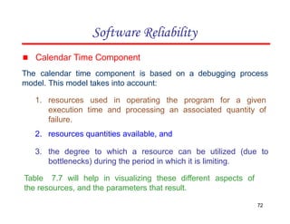
▪ Calendar TimeComponent
The calendar time component is based on a debugging process
model. This model takes into account:
1. resources used in operating the program for a given
execution time and processing an associated quantity of
failure.
2. resources quantities available, and
3. the degree to which a resource can be utilized (due to
bottlenecks) during the period in which it is limiting.
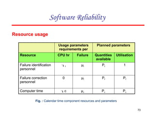
Table 7.7 will help in visualizing these different aspects of
the resources, and the parameters that result.
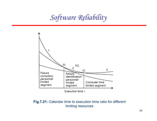
72
Software Reliability
73.
Software Reliability
73
Usage parameters
requirementsper
Planned parameters
Resource CPU hr Failure Quantities
available
Utilisation
Failure identification
personnel
I µI PI 1
Failure correction
personnel
0 µf Pf Pf
Computer time c µc Pc Pc
Fig. : Calendar time component resources and parameters
Resource usage
74.
Software Reliability
74
XC c
c
X f f
X I I
I
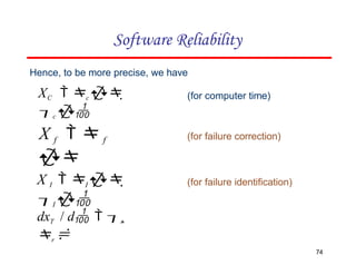
Hence, to be more precise, we have
(for computer time)
(for failure correction)
(for failure identification)
dxT / d r
r
Example- 7.4
A teamrun test cases for 10 CPU hrs and identifies 25 failures. The effort
required per hour of execution time is 5 person hr. Each failure requires 2
hr. on an average to verify and determine its nature. Calculate the failure
identification effort required.
Software Reliability
78
79.
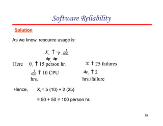
Solution
As we know,resource usage is:
Xr r
r
Software Reliability
79
θr 15 person hr.
10 CPU
hrs.
Here
Hence,
25 failures
r 2
hrs./failure
Xr = 5 (10) + 2 (25)
= 50 + 50 = 100 person hr.
80.
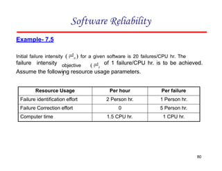
Example- 7.5
Initial failureintensity (0 ) for a given software is 20 failures/CPU hr. The
failure intensity objective (F
)
of 1 failure/CPU hr. is to be achieved.
Assume the following resource usage parameters.
Software Reliability
80
Resource Usage Per hour Per failure
Failure identification effort 2 Person hr. 1 Person hr.
Failure Correction effort 0 5 Person hr.
Computer time 1.5 CPU hr. 1 CPU hr.
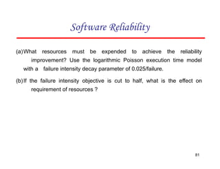
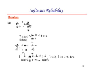
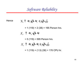
81.
(a)What resources mustbe expended to achieve the reliability
improvement? Use the logarithmic Poisson execution time model
with a failure intensity decay parameter of 0.025/failure.
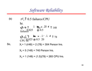
(b)If the failure intensity objective is cut to half, what is the effect on
requirement of resources ?
Software Reliability
81
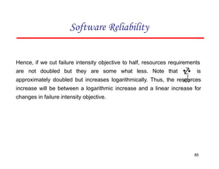
Hence, if wecut failure intensity objective to half, resources requirements
are not doubled but they are some what less. Note that is
approximately doubled but increases logarithmically. Thus, the resources
increase will be between a logarithmic increase and a linear increase for
changes in failure intensity objective.
Software Reliability
85
86.
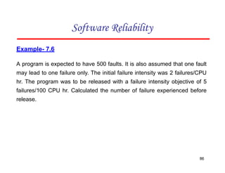
Example- 7.6
A programis expected to have 500 faults. It is also assumed that one fault
may lead to one failure only. The initial failure intensity was 2 failures/CPU
hr. The program was to be released with a failure intensity objective of 5
failures/100 CPU hr. Calculated the number of failure experienced before
release.
Software Reliability
86
87.
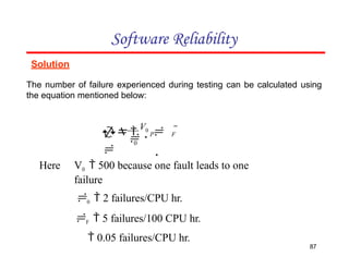
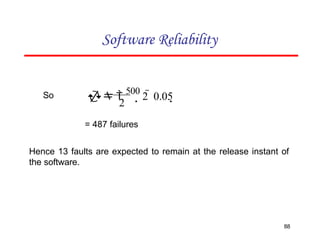
Solution
The number offailure experienced during testing can be calculated using
the equation mentioned below:
Software Reliability
P F
87
0
V0
V0 500 because one fault leads to one
failure
0 2 failures/CPU hr.
F 5 failures/100 CPU hr.
0.05 failures/CPU hr.
Here
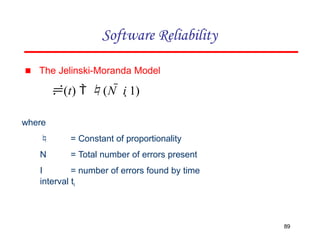
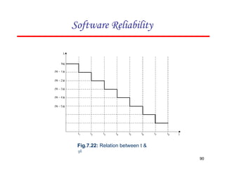
▪ The Jelinski-MorandaModel
(t) (N i 1)
where
= Constant of proportionality
N = Total number of errors present
I = number of errors found by time
interval ti
89
Software Reliability
Example- 7.7
There are100 errors estimated to be present in a program. We have
experienced 60 errors. Use Jelinski-Moranda model to calculate
failure intensity with a given value of =0.03. What will be
failure intensity after the experience of 80 errors?
Software Reliability
91
92.
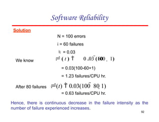
Solution
N = 100errors
i = 60 failures
= 0.03
Software Reliability
92
We know 60 1)
( t ) 0 .03 (100
= 0.03(100-60+1)
= 1.23 failures/CPU hr.
After 80 failures (t) 0.03(100 80 1)
= 0.63 failures/CPU hr.
Hence, there is continuous decrease in the failure intensity as the
number of failure experienced increases.
93.
Software Reliability
Nt nt
N Nt n nt
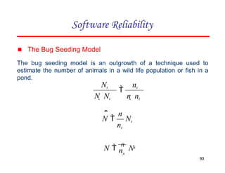
▪ The Bug Seeding Model
The bug seeding model is an outgrowth of a technique used to
estimate the number of animals in a wild life population or fish in a
pond.
Nt
nt
n
N
s
93
s
n
N
n
N
93
94.
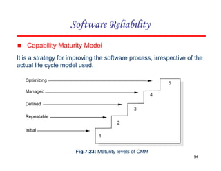
▪ Capability MaturityModel
It is a strategy for improving the software process, irrespective of the
actual life cycle model used.
Software Reliability
Fig.7.23: Maturity levels of CMM
94
Software Reliability
96
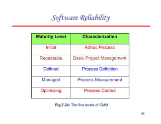
Fig.7.24: Thefive levels of CMM
Maturity Level Characterization
Initial Adhoc Process
Repeatable Basic Project Management
Defined Process Definition
Managed Process Measurement
Optimizing Process Control
97.
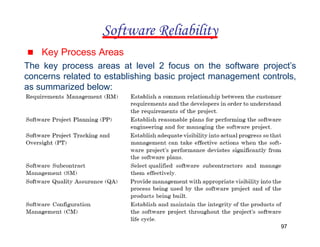
▪ Key ProcessAreas
The key process areas at level 2 focus on the software project’s
concerns related to establishing basic project management controls,
as summarized below:
Software Reliability
97
98.
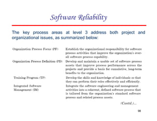
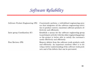
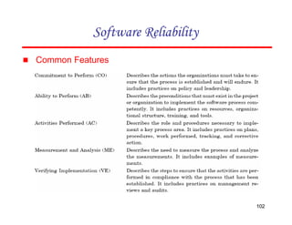
The key processareas at level 3 address both project and
organizational issues, as summarized below:
Software Reliability
98
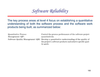
The key processareas at level 4 focus on establishing a quantitative
understanding of both the software process and the software work
products being built, as summarized below:
Software Reliability
100
101.
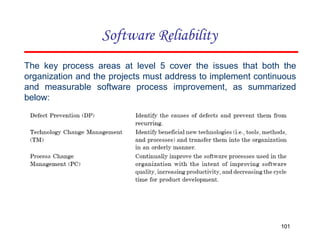
The key processareas at level 5 cover the issues that both the
organization and the projects must address to implement continuous
and measurable software process improvement, as summarized
below:
Software Reliability
101
▪ ISO 9000
TheSEI capability maturity model initiative is an attempt to improve
software quality by improving the process by which software is
developed.
ISO-9000 series of standards is a set of document dealing with
quality systems that can be used for quality assurance purposes.
ISO-9000 series is not just software standard. It is a series of five
related standards that are applicable to a wide variety of industrial
activities, including design/ development, production, installation,
and servicing. Within the ISO 9000 Series, standard ISO 9001 for
quality system is the standard that is most applicable to software
development.
103
Software Reliability
104.
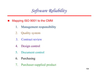
▪ Mapping ISO9001 to the CMM
1. Management responsibility
2. Quality system
3. Contract review
4. Design control
5. Document control
6. Purchasing
7. Purchaser-supplied product
Software Reliability
104
105.
8. Product identificationand traceability
9. Process control
10. Inspection and testing
11. Inspection, measuring and test equipment
12. Inspection and test status
13. Control of nonconforming product
14. Corrective action
Software Reliability
105
106.
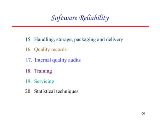
15. Handling, storage,packaging and delivery
16. Quality records
17. Internal quality audits
18. Training
19. Servicing
20. Statistical techniques
Software Reliability
106
107.
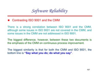
▪ Contrasting ISO9001 and the CMM
There is a strong correlation between ISO 9001 and the CMM,
although some issues in ISO 9001 are not covered in the CMM, and
some issues in the CMM are not addressed in ISO 9001.
The biggest difference, however, between these two documents is
the emphasis of the CMM on continuous process improvement.
The biggest similarity is that for both the CMM and ISO 9001, the
bottom line is “Say what you do; do what you say”.
107
Software Reliability
108.
(b) Useful life
(d)Test-out
(a) Burn-in
(c) Wear-out
7.2 Software reliability
is (a)the probability of failure free operation of a program for a specified
time in a specified environment
(b)the probability of failure of a program for a specified time in a
specified environment
(c)the probability of success of a program for a specified time in
any environment
(d) None of the above
7.3 Fault is
(b) Mistake in the program
(d) All of the above
(a) Defect in the program
(c) Error in the program
7.4 One fault may lead to
(a) one failure
(c) many failures
(b) two failures
(d) all of the above
Multiple Choice Questions
Note: Choose most appropriate answer of the following questions:
7.1 Which one is not a phase of “bath tub curve” of hardware reliability
108
109.
(b) 10
(d) 0
MultipleChoice Questions
7.5 Which ‘time’ unit is not used in reliability
studies
109
(a) Execution time
(c) Clock time
(b) Machine time
(d) Calendar time
7.6 Failure occurrences can be represented
as
(a) time to failure
(c) failures experienced in a time interval
(b) time interval between failures
(d) All of the above
7.9 As the reliability increases, failure
intensity
(a) decreases
(c) no effect
(b) increases
(d) None of the above
(b) 10
7.7 Maximum possible value of reliability
is
(a) 100
(c) 1
7.8 Minimum possible value of reliability is
(a) 100
(c) 1
(d) 0
110.
7.10 If failureintensity is 0.005 failures/hour during 10 hours of
operation of a software, its reliability can be expressed as
(b) 0.92
(d) 0.98
(a) 0.10
(c) 0.95
7.11 Software Quality is
(a) Conformance to requirements
(c) Level of satisfaction
7.12 Defect rate is
Multiple Choice Questions
(b) Fitness for the purpose
(d) All of the above
110
(a) number of defects per million lines of source code
(b) number of defects per function point
(c) number of defects per unit of size of software
(d) All of the above
7.13 How many product quality factors have been proposed in McCall quality
model?
(a) 2
(c) 11
(b) 3
(d) 6
111.
7.14 Which oneis not a product quality factor of McCall quality
model?
(a) Product revision
(c) Product specification
(b) Product operation
(d) Product transition
Multiple Choice Questions
7.15 The second level of quality attributes in McCall quality model are termed
as
111
(a) quality criteria
(c) quality guidelines
(b) quality factors
(d) quality specifications
7.16 Which one is not a level in Boehm software quality
model ?
(a) Primary uses
(c) Primitive constructs
(b) Intermediate constructs
(d) Final constructs
7.17 Which one is not a software quality
model?
(a) McCall model
(c) ISO 9000
(b) Boehm model
(d) ISO 9126
7.18 Basic execution time model was developed
by (a) Bev.Littlewood
(c) R.Pressman
(b) J.D.Musa
(d) Victor Baisili
112.
Multiple Choice Questions
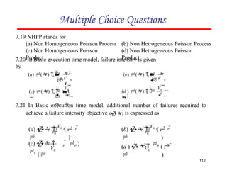
7.19NHPP stands for
(a) Non Homogeneous Poisson Process
(c) Non Homogeneous Poisson
Product
(b) Non Hetrogeneous Poisson Process
(d) Non Hetrogeneous Poisson
Product
7.20 In Basic execution time model, failure intensity is given
by
7.21 In Basic execution time model, additional number of failures required to
achieve a failure intensity objective () is expressed as
0
0
V
2
(a) ()
1
0
0
V
(b) ()
1
0
V0
(c) () 1
V0
2
0
(d ) ()
1
0
P F
(a)
V0
(
)
0
P
F
(b)
V0
(
)
0
P
)
F
V
(c)
0
(
0
112
F
P
V
(d )
0
(
)
113.
Multiple Choice Questions
7.22In Basic execution time model, additional time required to achieve a failure
intensity objective ( ) is given as
7.23 Failure intensity function of Logarithmic Poisson execution model is given
as
(a) () 0 LN
()
(c) () 0
exp()
F
V0
(c) Ln
P
0 P 0 F
V0
(d ) Ln
0 P
0
(a)
Ln V
113
F
P
0 F
0
(b)
Ln V
(b) () 0
exp()
(d ) () 0
log()
7.24 In Logarithmic Poisson execution model, ‘’ is known
as (a) Failure intensity function
parameter
(c) Failure intensity measurement
(b) Failure intensity decay parameter
(d) Failure intensity increment
parameter
114.
Multiple Choice Questions
7.25In jelinski-Moranda model, failure intensity is defined aseneous
Poisson Product
114
7.26 CMM level 1 has
(a) 6 KPAs
(c) 0 KPAs
7.27 MTBF stands for
(a) Mean time between failure
(c) Minimum time between failures
7.28 CMM model is a technique to
(a) Improve the software process
(c) Test the software
(b) 2 KPAs
(d) None of the above
(b) Maximum time between failures
(d) Many time between failures
(b) Automatically develop the software
(d) All of the above
7.29 Total number of maturing levels in CMM are
(a) 1
(c) 5
(b) 3
(d) 7
(a) (t) (N i
1)
(c) (t) (N i 1)
(b) (t) (N i
1)
(d ) (t) (N i
1)
115.
7.30 Reliability ofa software is dependent on number of errors
(a) removed
(c) both (a) & (b)
(b) remaining
(d) None of the above
7.31 Reliability of software is usually estimated at
(a) Analysis phase
(c) Coding phase
(b) Design phase
(d) Testing phase
Multiple Choice Questions
7.32 CMM stands for
(a) Capacity maturity model
(c) Cost management
model
115
(b) Capability maturity model
(d) Comprehensive maintenance
model
7.33 Which level of CMM is for basic project
management?
(a) Initial
(c) Defined
(b) Repeatable
(d) Managed
7.34 Which level of CMM is for process
management?
(a) Initial
(c) Defined
(b) Repeatable
(d) Optimizing
116.
Multiple Choice Questions
7.36CMM was developed at
(a) Harvard University
(c) Carnegie Mellon University
116
(b) Cambridge University
(d) Maryland University
7.39 The number of clauses used in ISO 9001
are (a) 15
(c) 20
(b) 25
(d) 10
7.35 Which level of CMM is for process
management?
(a) Initial
(c) Managed
(b) Defined
(d) Optimizing
7.38 The model to measure the software process improvement is
called
(a) ISO 9000
(c) CMM
(b) ISO 9126
(d) Spiral model
7.37 McCall has developed a
(a) Quality model
(c) Requirement model
(b) Process improvement model
(d) Design model
117.
Multiple Choice Questions
7.41In ISO 9126, each characteristics is related
to
117
(a) one attributes
(c) three attributes
(b) two attributes
(d) four attributes
7.44 Each maturity model is CMM
has
(a) One KPA
(c) Several KPAs
(b) Equal KPAs
(d) no KPA
7.40 ISO 9126 contains definitions
of
(a) quality characteristics
(c) quality attributes
(b) quality factors
(d) All of the above
7.43 Which is not a software reliability
model ?
(a) The Jelinski-Moranda Model
(c) Spiral model
(b) Basic execution time model
(d) None of the above
7.42 In McCall quality model; product revision quality factor consist
of (a) Maintainability
(c) Testability
(b) Flexibility
(d) None of the above
118.
Multiple Choice Questions
7.46In reliability models, our emphasis is
on
(a) errors
(c) failures
118
(b) faults
(d) bugs
7.49 MTTF stands for
(a) Mean time to failure
(c) Minimum time to failure
(b) Maximum time to failure
(d) None of the above
7.45 KPA in CMM stands for
(a) Key Process Area
(c) Key Principal Area
(b) Key Product Area
(d) Key Performance Area
7.48 Software reliability is defined with respect
to (a) time
(c) quality
(b) speed
(d) None of the above
7.47 Software does not break or wear out like hardware. What is your
opinion?
(a) True
(c) Can not say
(b) False
(d) not fixed
119.
Multiple Choice Questions
7.50ISO 9000 is a series of standards for quality management systems and
has
119
(a) 2 related standards
(c) 10 related standards
(b) 5 related standards
(d) 25 related standards
120.
Exercises
1. What issoftware reliability? Does it exist?
2. Explain the significance of bath tube curve of reliability with the help of
a diagram.
3. Compare hardware reliability with software reliability.
4. What is software failure? How is it related with a fault?
5. Discuss the various ways of characterising failure occurrences
with respect to time.
120
7.6 Describe the following terms:
(i) Operational profile
(iii) MTBF
(v) Failure intensity.
(ii)
(iv)
Input space
MTTF
121.
Exercises
7. What areuses of reliability studies? How can one use software reliability
measures to monitor the operational performance of software?
8. What is software quality? Discuss software quality attributes.
9. What do you mean by software quality standards? Illustrate their essence
as well as benefits.
10. Describe the McCall software quality model. How many product
quality factors are defined and why?
11. Discuss the relationship between quality factors and quality criteria
in McCall’s software quality model.
12. Explain the Boehm software quality model with the help of a
block diagram.
13. What is ISO9126 ? What are the quality characteristics and attributes?
121
122.
Exercises
7.14 Compare theISO9126 with McCall
software quality model and highlight few advantages of
ISO9126.
122
7.15 Discuss the basic model of software reliability. How
calculated.
can be
7.16 Assume that the initial failure intensity is 6 failures/CPU hr. The failure
intensity decay parameter is 0.02/failure. We assume that 45 failures
have been experienced. Calculate the current failure intensity.
7.17 Explain the basic & logarithmic Poisson model and their significance in
reliability studies.
and
123.
Exercises
7.18 Assume thata program will experience 150 failures in infinite time. It
has now experienced 80. The initial failure intensity was 10 failures/CPU
hr.
(i) Determine the current failure intensity
(ii)Calculate the failures experienced and failure intensity after 25
and 40 CPU hrs. of execution.
(iii)Compute additional failures and additional execution time
required to reach the failure intensity objective of 2 failures/CPU hr.
Use the basic execution time model for the above
mentioned calculations.
7.19 Write a short note on Logarithmic Poisson Execution time model. How
can we calculate & ?
7.20 Assume that the initial failure intensity is 10 failures/CPU hr. The
failure intensity decay parameter is 0.03/failure. We have experienced 75
failures upto this time. Find the failures experienced and failure intensity
after 25 and 50 CPU hrs. of execution.
123
124.
Exercises
7.21 The followingparameters for basic and logarithmic Poisson models are
given:
Determine the additional failures and additional execution time required
to reach the failure intensity objective of 0.1 failure/CPU hr. for both
models.
7.22 Quality and reliability are related concepts
but are fundamentally different in a number of ways. Discuss
them.
7.23 Discuss the calendar time component model. Establish the relationship
between calendar time to execution time.
124
125.
Exercises
24. A programis expected to have 250 faults. It is also assumed that
one fault may lead to one failure. The initial failure intensity is 5
failure/CPU hr. The program is released with a failure intensity
objective of 4 failures/10 CPU hr. Calculate the number of failures
experienced before release.
25. Explain the Jelinski-Moranda model of reliability theory. What is
the relation between ‘t’ and ' ' ?
26. Describe the Mill’s bug seeding model. Discuss few advantages of
this model over other reliability models.
27. Explain how the CMM encourages continuous improvement of
the software process.
28. Discuss various key process areas of CMM at various maturity levels.
29. Construct a table that correlates key process areas (KPAs) in the
CMM with ISO9000.
30. Discuss the 20 clauses of ISO9001 and compare with the practices in
the CMM.
125
126.
Exercises
31. List thedifference of CMM and ISO9001. Why is it suggested
that CMM is the better choice than ISO9001?
32. Explain the significance of software reliability engineering. Discuss
the advantage of using any software standard for software development?
33. What are the various key process areas at defined level in
CMM? Describe activities associated with one key process area.
34. Discuss main requirements of ISO9001 and compare it with
SEI capability maturity model.
35. Discuss the relative merits of ISO9001 certification and the SEI
CMM based evaluation. Point out some of the shortcomings of the
ISO9001 certification process as applied to the software industry.
126