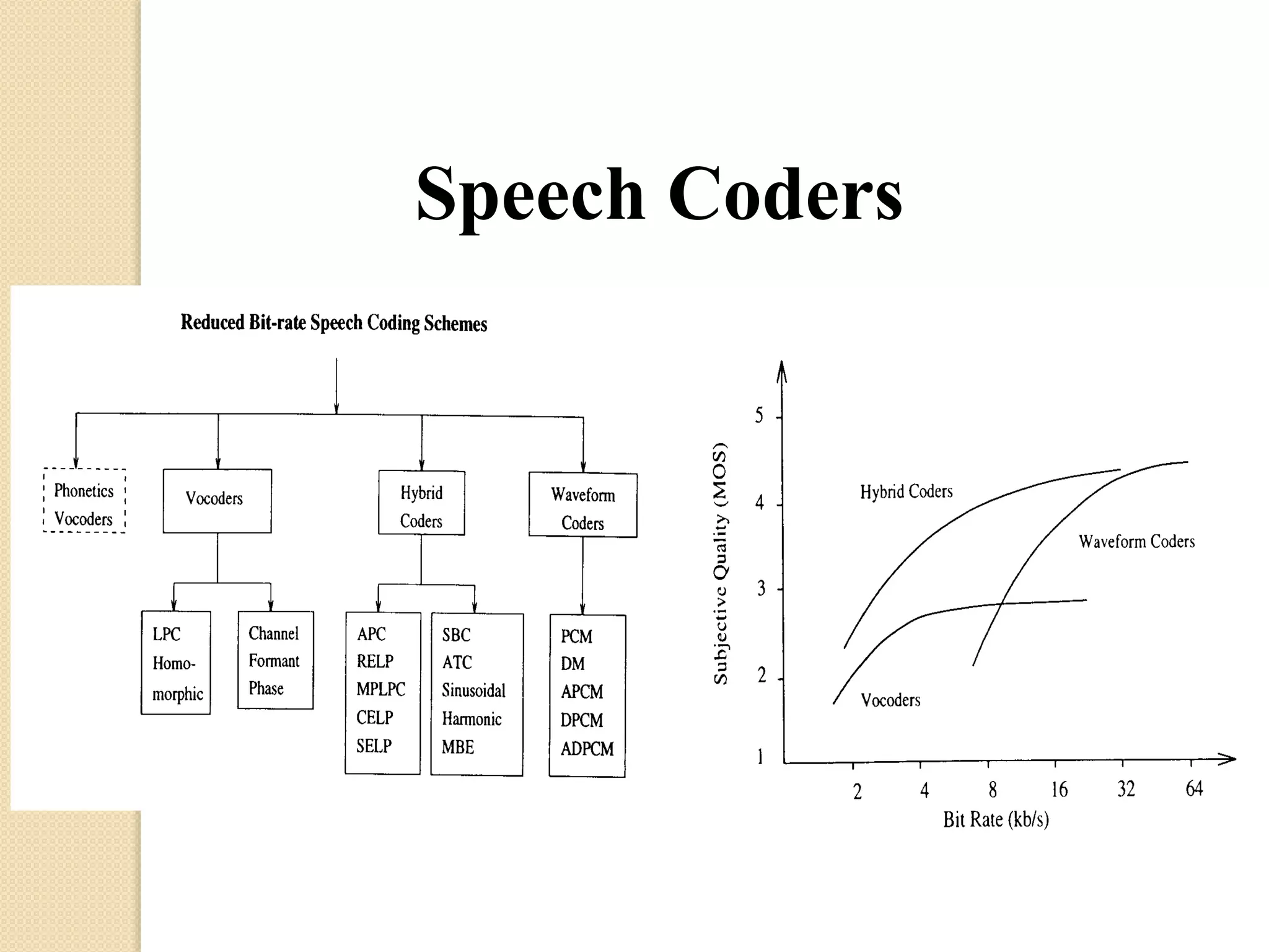
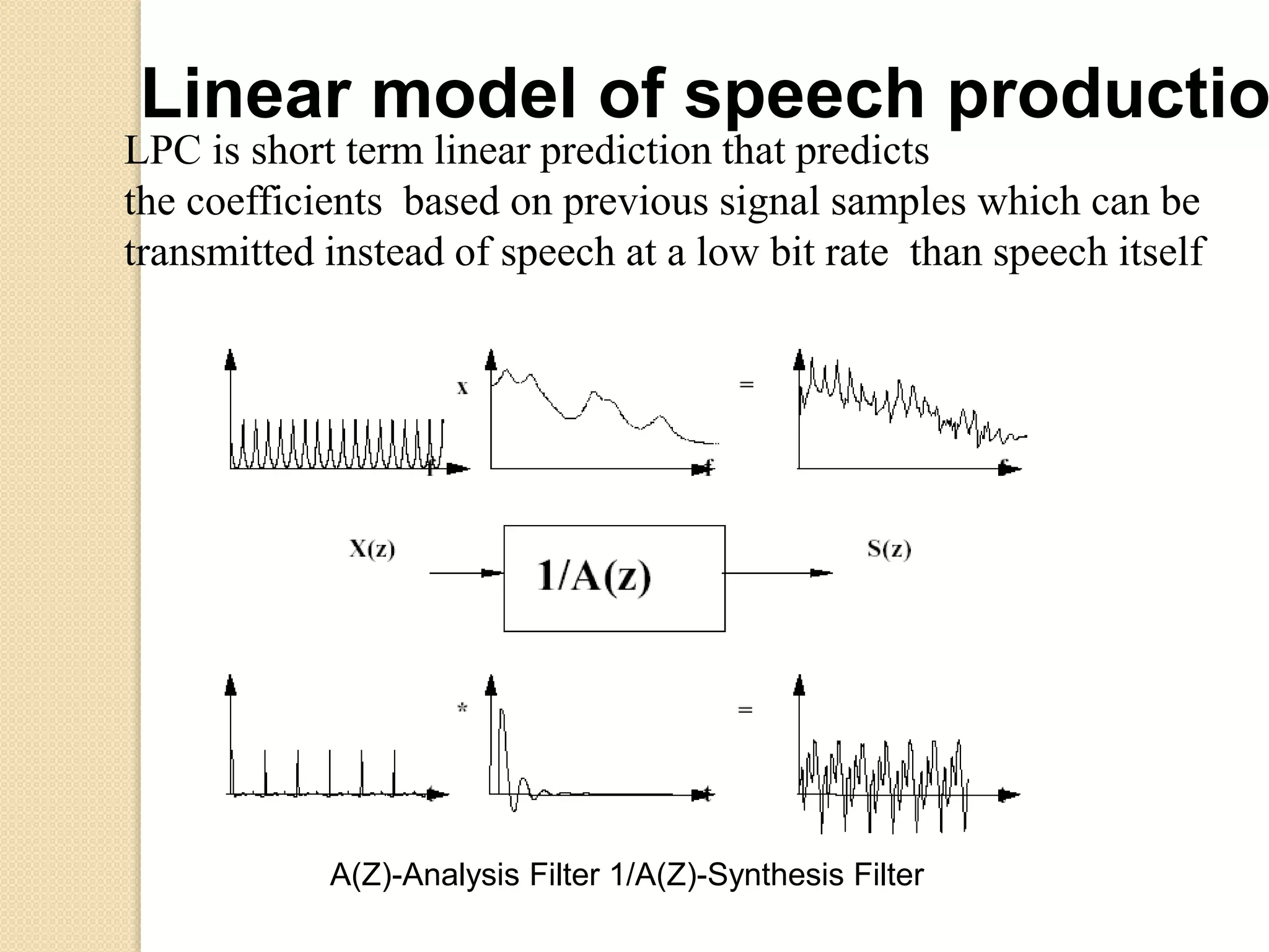
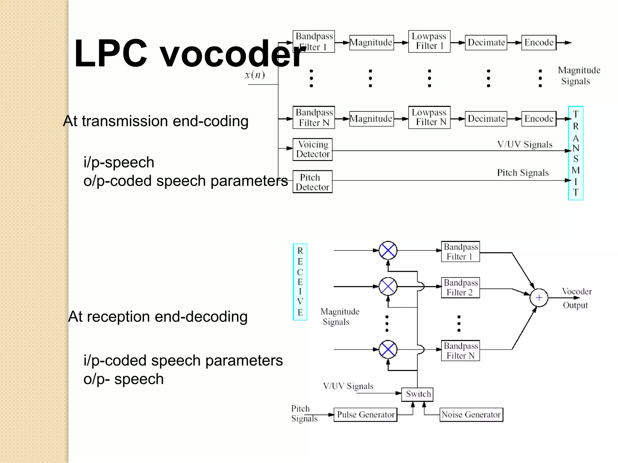
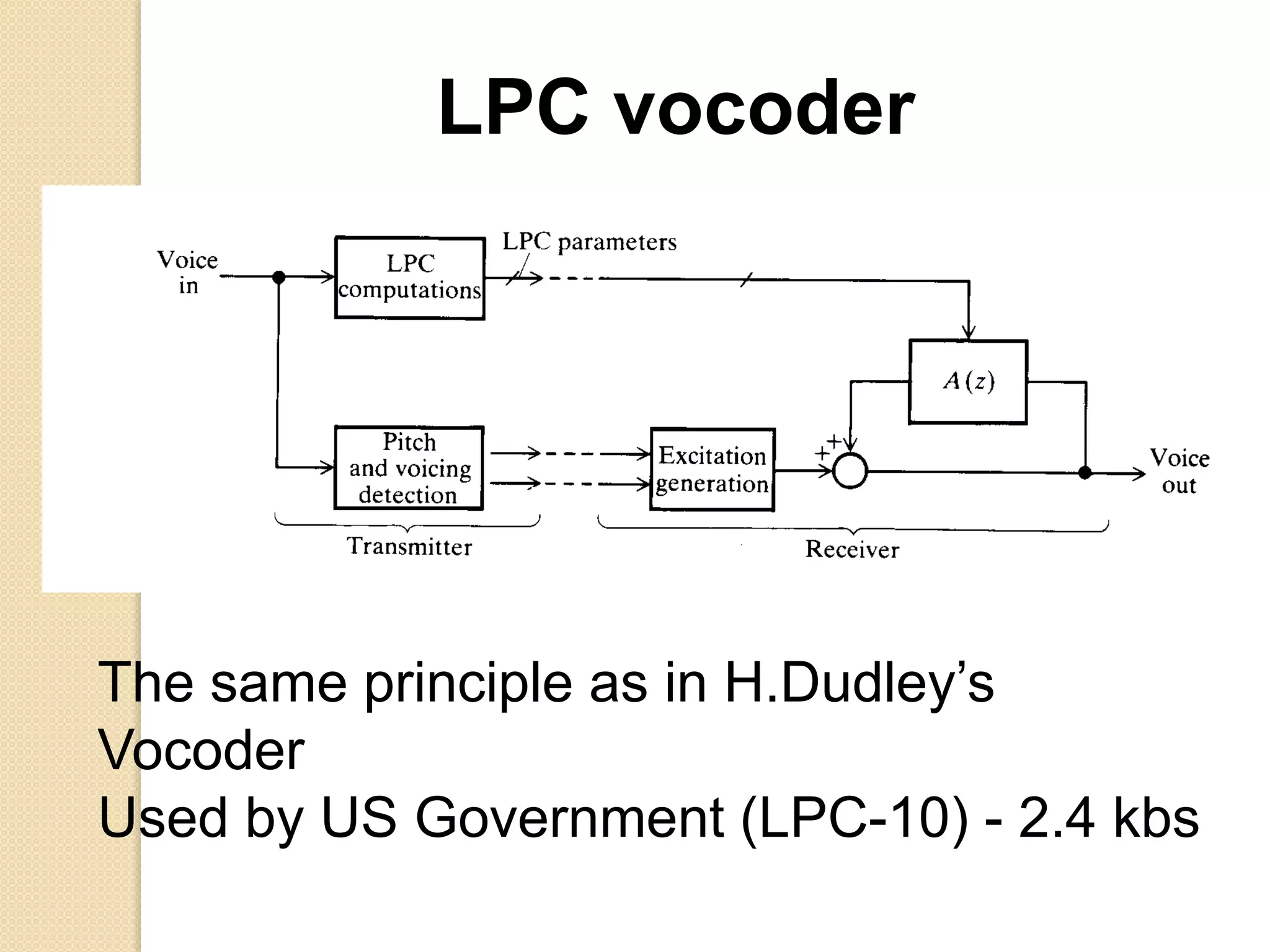
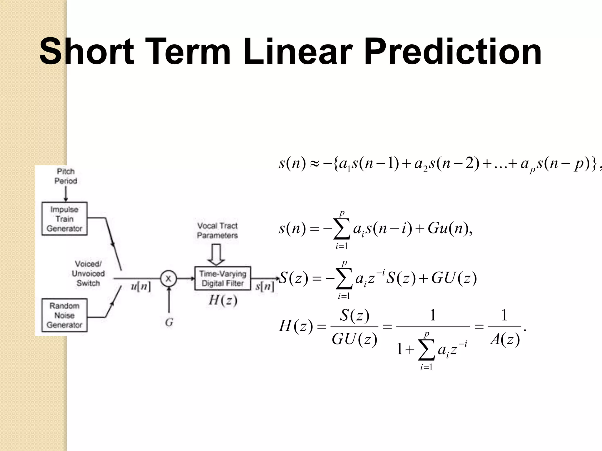
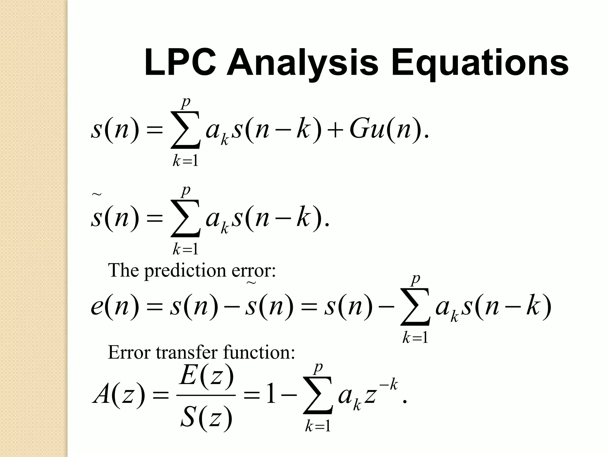
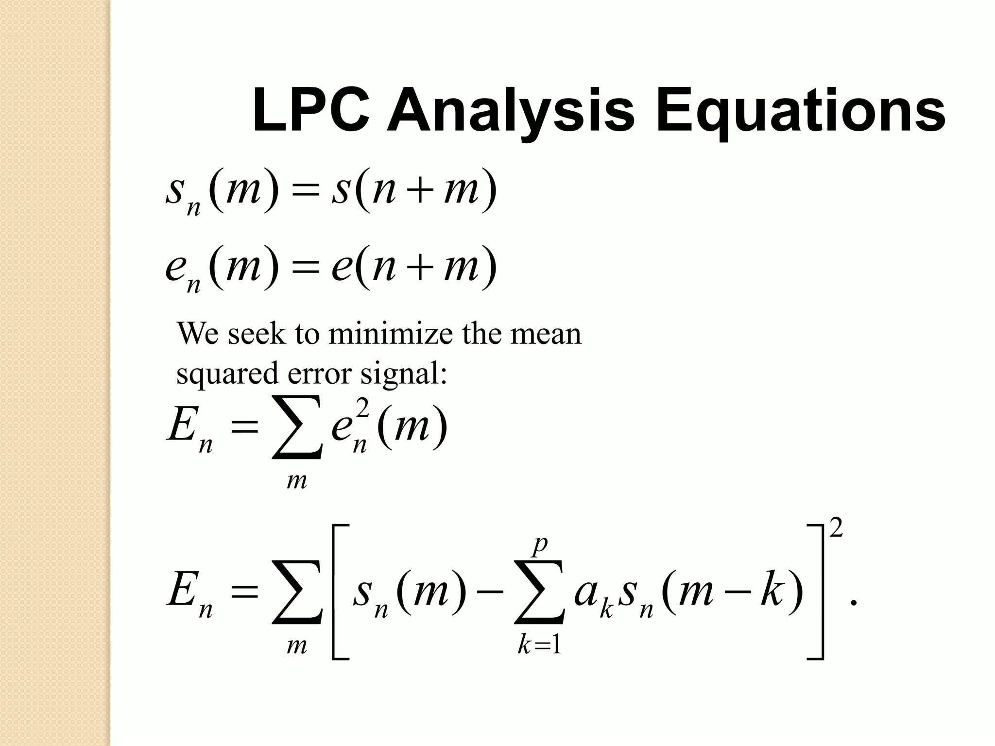
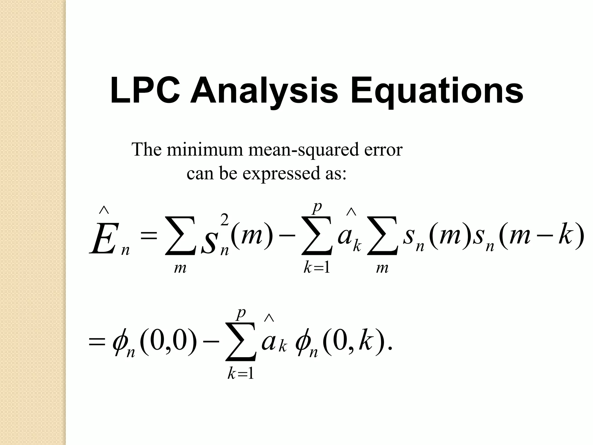
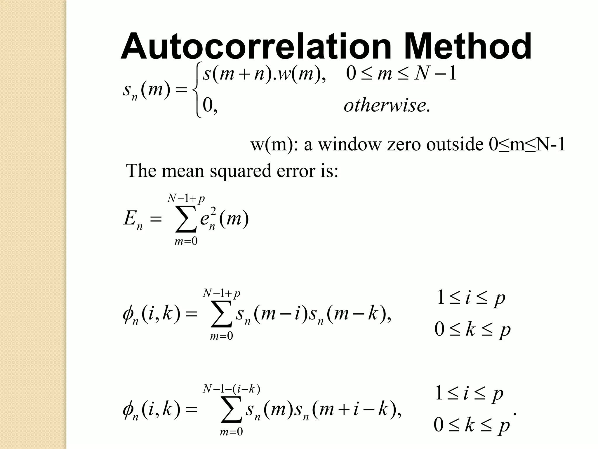
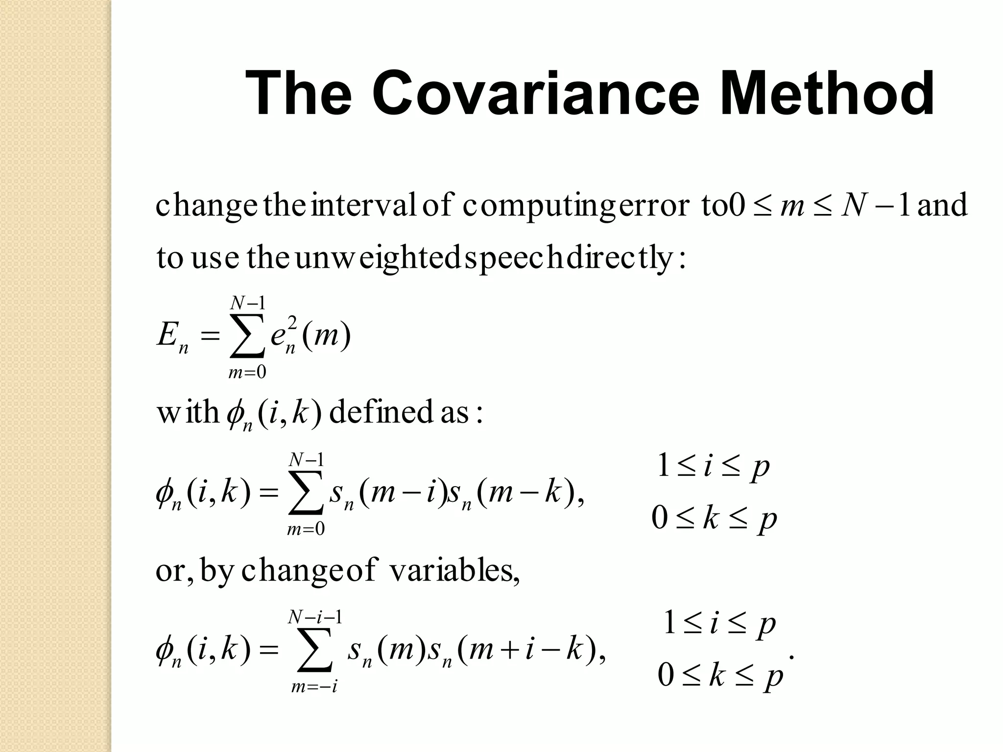
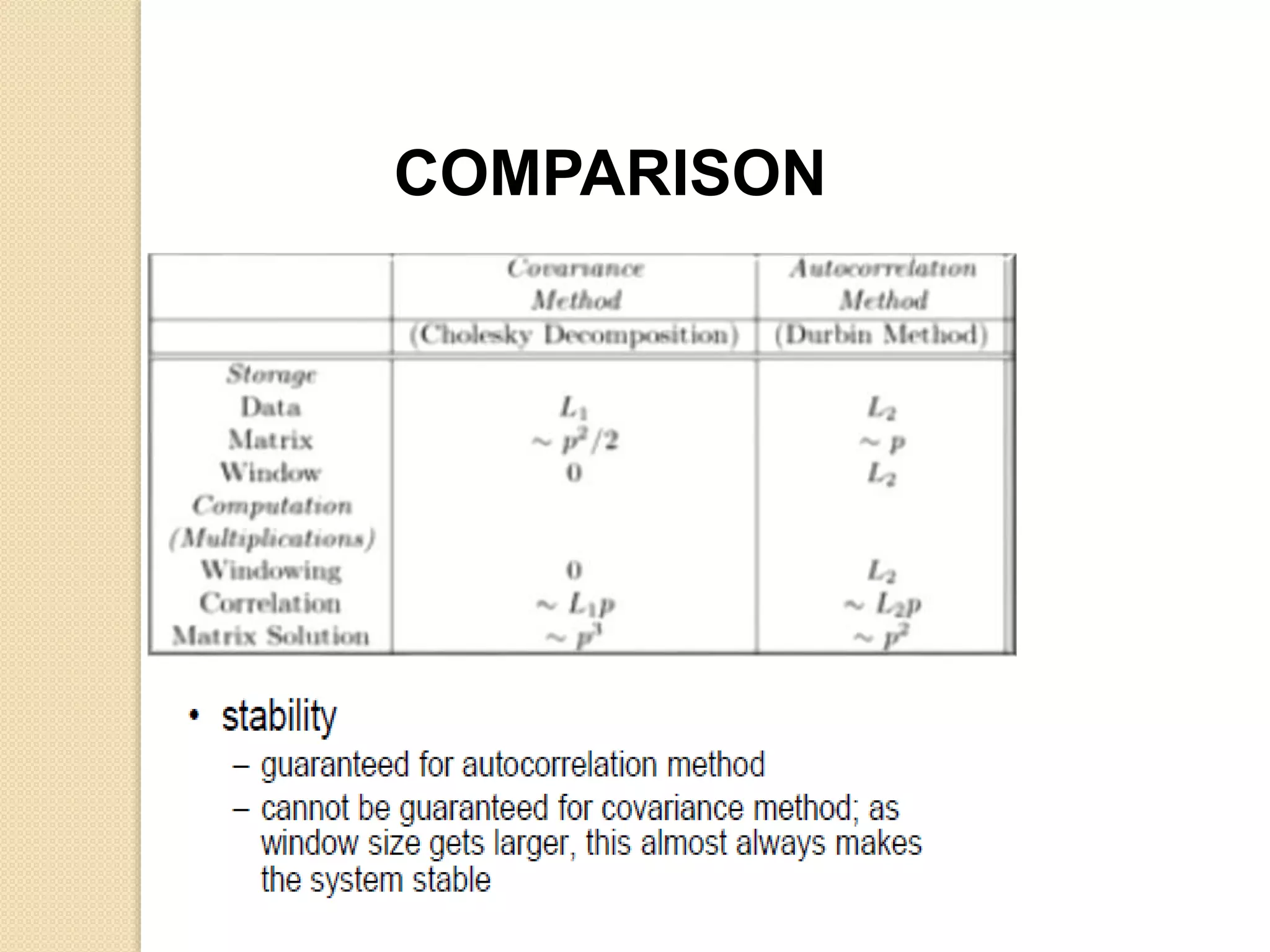
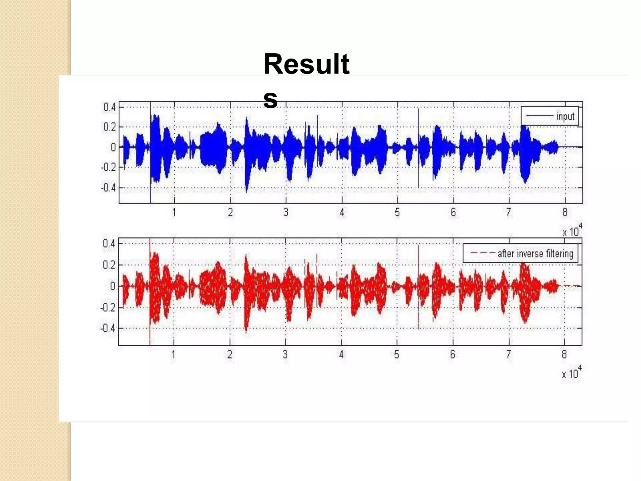
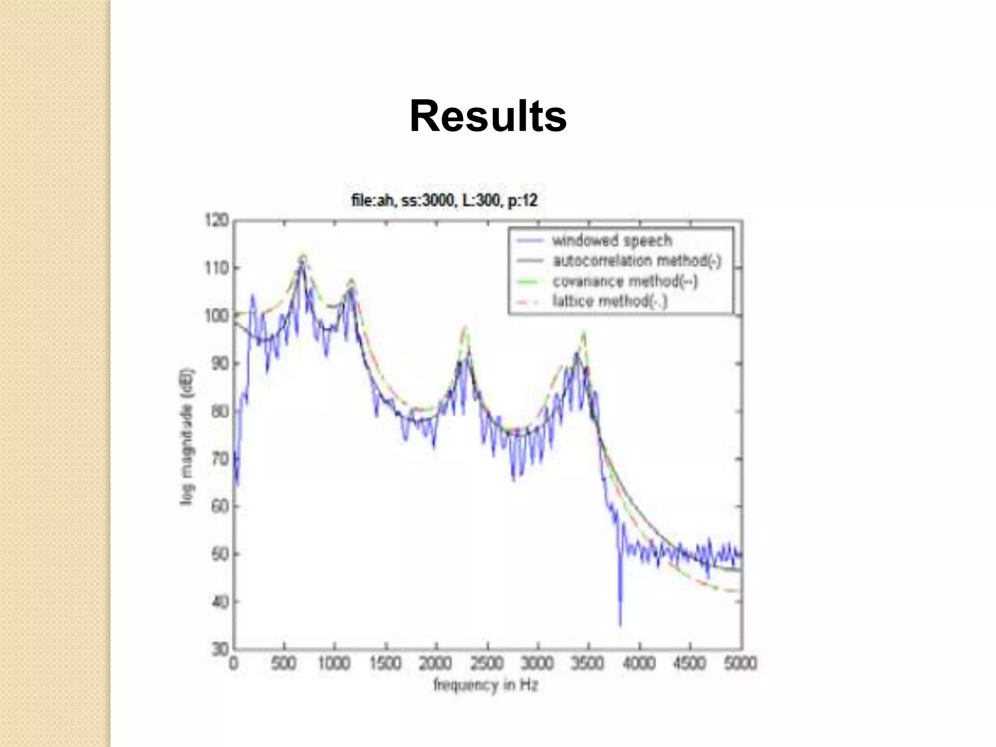
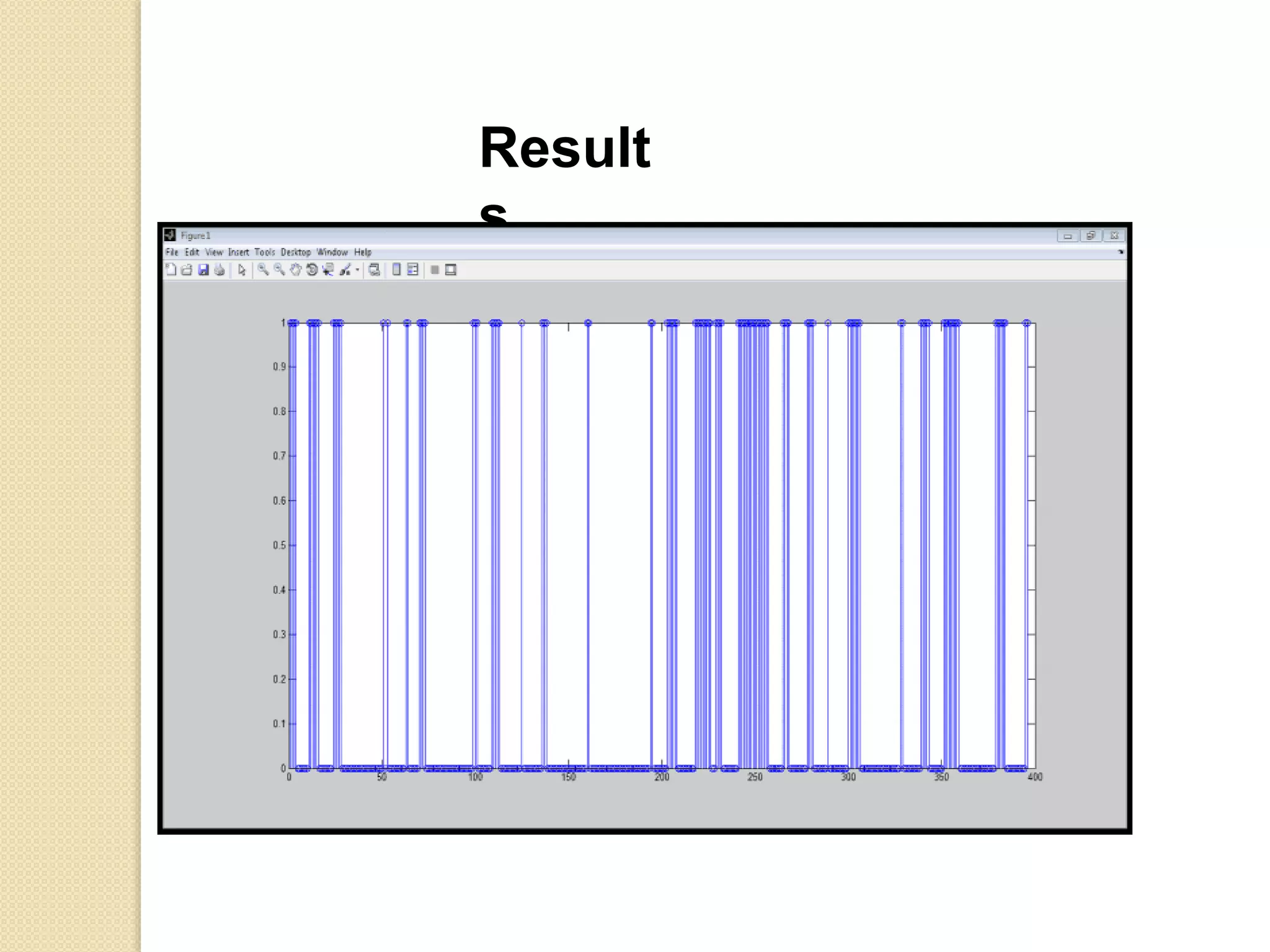
LINEAR PREDICTIVE
CODING METHODS AND
HORN NOISE DETECTION
By
P GOPIKRISHNA (12)
EASHWAR JEEVAN(15)
V V N PRANATHI(30)
• Introduction to speech coders.
• Speech production and
modeling(coding).
• Basic Principles of Linear Predictive
Analysis.
• The Autocorrelation Method.
• The Covariance Method.
• Solution of the LPC Equations.
• Horn noise detection using LPC
Contents
Speech Coders
Waveform Codec
• Waveform codec’s attempt, without using any
knowledge of how the signal to be coded was
generated, to produce a reconstructed signal
whose waveform is as close as possible to the
original.
• This means that in theory they should be signal
independent and work well with non-speech
signals.
• Generally they are low complexity codec’s which
produce high quality speech at rates above about
16 kbits/s.
• When the data rate is lowered below this level
the reconstructed speech quality that can be
obtained degrades rapidly
Source Codec
• Source coders operate using a model of how the source
was generated, and attempt to extract, from the signal
being coded, the parameters of the model.
• It is these model parameters which are transmitted to the
decoder.
• Source coders for speech are called vocoders, and work
as follows.
• The vocal tract is represented as a time-varying filter and
is excited with either a white noise source, for unvoiced
speech segments, or a train of pulses separated by the
pitch period for voiced speech.
• Therefore the information which must be sent to the
decoder is the filter specification, a voiced/unvoiced flag,
the necessary variance of the excitation signal, and the
pitch period for voiced speech.
Desirable Properties of a
Speech Coder
• Low Bit-Rate
• High Speech Quality
• Robustness Across Different Speakers / Languages
• Robustness in the Presence of Channel Errors
• Good Performance on Nonspeech Signals
• Low Memory Size and Low Computational
Complexity
• Low Coding Delay
Applications of Speech Coding
 Digital Transmissions
◦ On wired telephone:
 Multiplexing
 Integration of services
◦ On wireless channels:
 Spectral efficiency
 For better protection against errors
 Voice mail/messaging
 Storage: telephone answering machine
 Secure phone
•study human hearing, especially
masking
•speech production mechanism
•speaker characteristics
•linguistic code (recognition-synthesis)
•thought-to-speech
Future in speech
coding
Speech production and
modeling
Speech Signal
Speech Spectrum for a Voiced
Sound
current
sample
time
short-term prediction
short-term - resonance of vocal tract
long-term - periodicity of voiced speech
(vocal cord vibration)
long-term prediction
source filter speech
log spectrum
LPC is short term linear prediction that predicts
the coefficients based on previous signal samples which can be
transmitted instead of speech at a low bit rate than speech itself
Linear model of speech productio
A(Z)-Analysis Filter 1/A(Z)-Synthesis Filter
At transmission end-coding
At reception end-decoding
i/p-speech
o/p-coded speech parameters
i/p-coded speech parameters
o/p- speech
LPC vocoder
The same principle as in H.Dudley’s
Vocoder
Used by US Government (LPC-10) - 2.4 kbs
LPC vocoder
Short Term Linear Prediction
• The coefficients of H(z)=1/A(z) can be
obtained by linear prediction.
• Short term analysis on x(n) speech signal
– Frames of 10 to 30 ms.
• Least square error criterion
.
)(
1
1
1
)(
)(
)(
)()()(
,)()()(
)},(...)2()1({)(
1
1
1
21
zA
za
zGU
zS
zH
zGUzSzazS
nGuinsans
pnsansansans
p
i
i
i
p
i
i
i
p
i
i
p














Short Term Linear Prediction
.1
)(
)(
)(
)()()()()(
).()(
).()()(
1
1
~
1
~
1













p
k
k
k
p
k
k
p
k
k
p
k
k
za
zS
zE
zA
knsansnsnsne
knsans
nGuknsans
LPC Analysis Equations
Error transfer function:
The prediction error:
.)()(
)(
)()(
)()(
2
1
2
 











m
p
k
nknn
m
nn
n
n
kmsamsE
meE
mneme
mnsms
We seek to minimize the mean
squared error signal:
LPC Analysis Equations








p
k
nkn
m
nn
p
k
k
m
nn
ka
kmsmsamsE
1
1
2
).,0()0,0(
)()()(

The minimum mean-squared error
can be expressed as:
LPC Analysis Equations
.
0
1
),()(),(
0
1
),()(),(
)(
.,0
10),().(
)(
)(1
0
1
0
1
0
2
pk
pi
kimsmski
pk
pi
kmsimski
meE
otherwise
Nmmwnms
ms
kiN
m
nnn
pN
m
nnn
pN
m
nn
n









 












Autocorrelation Method
w(m): a window zero outside 0≤m≤N-1
The mean squared error is:
Autocorrelation Method
)(),(
:functionationautocorrelsimpletoreducesfunction
covariancethek,-ioffunctionaonlyis),(Since
.
0
1
),()(),(
)(1
0
kirki
ki
pk
pi
kimsmski
nn
n
kin
m
nnn



 





.
)(
)3(
)2(
)1(
)0(...)3()2()1(
)3(...)0()1()2(
)2(...)1()0()1(
)1(...)2()1()0(
:asformmatrixinexpressedbecanand
1),(|)(|
:)()(i.e.
symmetric,isfunctionationautocorreltheSince
2
1
1



















































pr
r
r
r
a
a
a
rprprpr
prrrr
prrrr
prrrr
piirakir
sokrkr
n
n
n
n
pnnnn
nnnn
nnnn
nnnn
p
k
nkn
nn
Autocorrelation Method
Levinson Durbin algorithm is often used to
solve these equations by using the
properties of toeplitz matrix and linear
prediction
Autocorrelation Method

















1
1
0
1
0
2
.
0
1
),()(),(
,variablesofchangebyor,
0
1
),()(),(
:asdefined),(with
)(
:directlyspeechunweightedtheuseto
and10error tocomputingofintervalthechange
iN
im
nnn
n
N
m
nn
n
N
m
nn
pk
pi
kimsmski
pk
pi
kmsimski
ki
meE
Nm



The Covariance Method
.
)0,(
)0,3(
)0,2(
)0,1(
),()3,()2,()1,(
),3()3,3()2,3()1,3(
),2()3,2()2,2()1,2(
),1()3,1()2,1()1,1(
3
2
1























































pa
a
a
a
ppppp
p
p
p
n
n
n
n
p
nnnn
nnnn
nnnn
nnnn














The resulting covariance matrix is symmetric, but not
Toeplitz, and can be solved efficiently by a set of techniques
called Cholesky decomposition
The Covariance Method
Autocorrelation/Covariance
Summary
1.Autocorrelation Method => signal is windowed by a taperin
window in order to minimize discontinuities at beginning
(predicting speech from zero-valued samples) and end
(predicting zero-valued samples from speech samples) of the
interval
2. Covariance method => the signal is extended by p samples
outside the normal range of to include p
samples occurring prior to m=0 (they are available) and
eliminates the need for a tapering window; resulting matrix of
correlations is symmetric
COMPARISON
Result
s
Results
•we have added a speech signal and
known horn noise .
• Threshold value observed practically for
given horn noise.
•LPC residue for horn and silence is low whereas for
speech it is high.
•The above property is used to develop algorithm to
detect horn noise.
Horn noise detection
Result
s
Softwares:
REFERENCES:
•SPEECH CODING ALGORITHMS Foundation and Evolution
of Standardized Coders -WAI C. CHU
•Lecture Notes in Speech Production, Speech Coding, and
Speech Recognition Mark Hasegawa-Johnson of University of
Illinois
•Introduction to Speech Processing | Ricardo Gutierrez-Osuna |
CSE TAMU(Texas A & M U niversity)
Linear Predictive Coding, Jeremy Bradbury, December 5, 2000
lpc and horn noise detection

lpc and horn noise detection