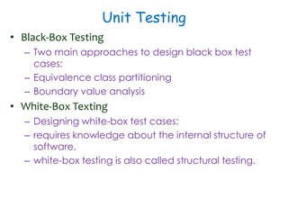
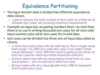
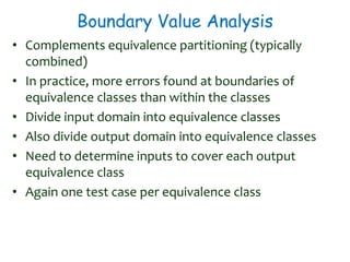
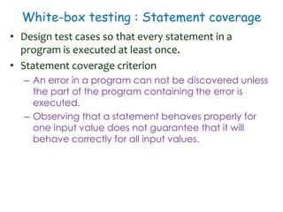
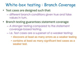
Software Engineering Principles
Ajit K Nayak, Ph.D.
ajitnayak@soauniversity.ac.in
Software Testing
Acknowledgements
• Slides of Prof. Rajib Mall, IIT, KGP
Unit Testing
• Black-Box Testing
– Two main approaches to design black box test
cases:
– Equivalence class partitioning
– Boundary value analysis
• White-Box Texting
– Designing white-box test cases:
– requires knowledge about the internal structure of
software.
– white-box testing is also called structural testing.
Equivalence Partitioning
• The input domain data is divided into different equivalence
data classes.
– used to reduce the total number of test cases to a finite set of
testable test cases, still covering maximum requirements.
• Example: an input box accepting numbers from 1 to 1000 then
there is no use in writing thousand test cases for all 1000 valid
input numbers plus other test cases for invalid data.
• test cases can be divided into three sets of input data called as
classes.
– 1) One input data class with all valid inputs. Pick a single value
from range 1 to 1000 as a valid test case. If you select other
values between 1 and 1000 then result is going to be same. So
one test case for valid input data should be sufficient.
– 2) Input data class with all values below lower limit. I.e. any
value below 1, as a invalid input data test case.
– 3) Input data with any value greater than 1000 to represent
third invalid input class.
Boundary Value Analysis
• Complements equivalence partitioning (typically
combined)
• In practice, more errors found at boundaries of
equivalence classes than within the classes
• Divide input domain into equivalence classes
• Also divide output domain into equivalence classes
• Need to determine inputs to cover each output
equivalence class
• Again one test case per equivalence class
White-box testing : Statement coverage
• Design test cases so that every statement in a
program is executed at least once.
• Statement coverage criterion
– An error in a program can not be discovered unless
the part of the program containing the error is
executed.
– Observing that a statement behaves properly for
one input value does not guarantee that it will
behave correctly for all input values.
Example: Euclid's GCD Algorithm
int f1(int x, int y){
1 while (x != y){
2 if (x>y) then
3 x=x-y;
4 else
5 y=y-x;
5 }
6 return x;
}
• By choosing the
test set
• {(x=3,y=3),
• (x=4,y=3),
• (x=3,y=4)}
• all statements are
executed at least
once.
White-box testing : Branch Coverage
• Test cases are designed such that:
– different branch conditions given true and false
values in turn.
• Branch testing guarantees statement coverage:
– A stronger testing compared to the statement
coverage-based testing.
– i.e. Test cases are a superset of a weaker testing:
• discovers at least as many errors as a weaker testing
• contains at least as many significant test cases as a
weaker test.
Example: Euclid's GCD Algorithm
int f1(int x, int y){
1 while (x != y){
2 if (x>y) then
3 x=x-y;
4 else
5 y=y-x;
5 }
6 return x;
}
• Test cases for
branch coverage
can be:
• {(x=3,y=3),
• (x=3,y=2),
• (x=4,y=3),
• (x=3,y=4)}
White-box Testing: Condition Coverage
• Test cases are designed such that:
– each component of a composite conditional
expression
– given both true and false values.
• Consider the conditional expression
– ((c1.and.c2).or.c3):
– Each of c1, c2, and c3 are exercised at least
once, i.e. given true and false values.
• It require 2n (the number of component conditions)
test cases.
– practical only if n is small
White-box testing : Path Coverage
• Design test cases such that:
– all linearly independent paths in the program are
executed at least once.
• Defined in terms of control flow graph (CFG) of a
program.
• A control flow graph (CFG) describes:
– the sequence in which different instructions of a
program get executed.
– the way control flows through the program.
Drawing a CFG - I
• Number all the statements of a program.
– Numbered statements represent nodes of the
control flow graph.
• An edge from one node to another node exists:
– if execution of the statement representing the first
node can result in transfer of control to the other
node.
• Sequence:
– 1 a=5;
– 2 b=a*b-1;
1
2
Drawing a CFG - II
• Selection:
1. if(a>b) then
2. c=3;
3. else
4. c=5;
5. c=c*c;
• Iteration:
• 1 while(a>b){
• 2 b=b*a;
• 3 b=b-1;}
• 4 c=b+d;
1
2 3
4
1
2
3
4
Example
int f1(int x, int y){
1 while (x != y){
2 if (x>y) then
3 x=x-y;
4 else
5 y=y-x;
5 }
6 return x;
}
1
2
3 4
5
6
Path
• A path through a program:
– a node and edge sequence from the starting node
to a terminal node of the control flow graph.
• There may be several terminal nodes for program.
• Any path through the program:
• introducing at least one new node that is not included
in any other independent paths.
• McCabe's cyclomatic metric is an upper bound:
– for the number of linearly independent paths of a
program
• Provides a practical way of determining the maximum
number of linearly independent paths in a program.
Cyclomatic Complexity - I
• Given a control flow graph G, cyclomatic complexity
V(G) = E-N+2
– N is the number of nodes in G
– E is the number of edges in G
• Cyclomatic complexity = 7-6+2 = 3. 1
2
3 4
5
6
• Another way of computing
cyclomatic complexity:
• determine number of bounded
areas in the graph
• V(G) = Total number of bounded
areas + 1
• Example: the number of bounded
areas is 2.
• Cyclomatic complexity = 2+1=3.
Cyclomatic Complexity - II
• The cyclomatic complexity of a program provides a
lower bound on the number of test cases to be
designed
– to guarantee coverage of all linearly independent
paths.
– does not make it any easier to derive the test cases,
– only gives an indication of the minimum number of
test cases required.
Path Testing
• Draw control flow graph.
• Determine V(G).
• Determine the set of linearly
independent paths.
• Prepare test cases:
• to force execution along each
path.
• Number of independent paths: 3
• 1,6 test case (x=1, y=1)
• 1,2,3,5,1,6 test case(x=1, y=2)
• 1,2,4,5,1,6 test case(x=2, y=1)
1
2
3 4
5
6
Cyclomatic Complexity - III
• Relationship exists between
– McCabe's metric & the number of errors existing in
the code,
– the time required to find and correct the errors.
• also indicates the psychological complexity of a
program.
• i.e. difficulty level of understanding the program.
• Therefore, limit cyclomatic complexity of modules to
some reasonable value. (10 or so)
Automated Testing Tools
• Mercury Interactive
• Quick Test Professional: Regression testing
• WinRunner: UI testing
• IBM Rational
• Rational Robot
• Functional Tester
• Borland
• Silk Test
• Compuware
• QA Run
• AutomatedQA
• TestComplete
Thank You

Software Engineering : Software testing

  • 1.
    Software Engineering Principles AjitK Nayak, Ph.D. ajitnayak@soauniversity.ac.in Software Testing
  • 2.
    Acknowledgements • Slides ofProf. Rajib Mall, IIT, KGP
  • 3.
    Unit Testing • Black-BoxTesting – Two main approaches to design black box test cases: – Equivalence class partitioning – Boundary value analysis • White-Box Texting – Designing white-box test cases: – requires knowledge about the internal structure of software. – white-box testing is also called structural testing.
  • 4.
    Equivalence Partitioning • Theinput domain data is divided into different equivalence data classes. – used to reduce the total number of test cases to a finite set of testable test cases, still covering maximum requirements. • Example: an input box accepting numbers from 1 to 1000 then there is no use in writing thousand test cases for all 1000 valid input numbers plus other test cases for invalid data. • test cases can be divided into three sets of input data called as classes. – 1) One input data class with all valid inputs. Pick a single value from range 1 to 1000 as a valid test case. If you select other values between 1 and 1000 then result is going to be same. So one test case for valid input data should be sufficient. – 2) Input data class with all values below lower limit. I.e. any value below 1, as a invalid input data test case. – 3) Input data with any value greater than 1000 to represent third invalid input class.
  • 5.
    Boundary Value Analysis •Complements equivalence partitioning (typically combined) • In practice, more errors found at boundaries of equivalence classes than within the classes • Divide input domain into equivalence classes • Also divide output domain into equivalence classes • Need to determine inputs to cover each output equivalence class • Again one test case per equivalence class
  • 6.
    White-box testing :Statement coverage • Design test cases so that every statement in a program is executed at least once. • Statement coverage criterion – An error in a program can not be discovered unless the part of the program containing the error is executed. – Observing that a statement behaves properly for one input value does not guarantee that it will behave correctly for all input values.
  • 7.
    Example: Euclid's GCDAlgorithm int f1(int x, int y){ 1 while (x != y){ 2 if (x>y) then 3 x=x-y; 4 else 5 y=y-x; 5 } 6 return x; } • By choosing the test set • {(x=3,y=3), • (x=4,y=3), • (x=3,y=4)} • all statements are executed at least once.
  • 8.
    White-box testing :Branch Coverage • Test cases are designed such that: – different branch conditions given true and false values in turn. • Branch testing guarantees statement coverage: – A stronger testing compared to the statement coverage-based testing. – i.e. Test cases are a superset of a weaker testing: • discovers at least as many errors as a weaker testing • contains at least as many significant test cases as a weaker test.
  • 9.
    Example: Euclid's GCDAlgorithm int f1(int x, int y){ 1 while (x != y){ 2 if (x>y) then 3 x=x-y; 4 else 5 y=y-x; 5 } 6 return x; } • Test cases for branch coverage can be: • {(x=3,y=3), • (x=3,y=2), • (x=4,y=3), • (x=3,y=4)}
  • 10.
    White-box Testing: ConditionCoverage • Test cases are designed such that: – each component of a composite conditional expression – given both true and false values. • Consider the conditional expression – ((c1.and.c2).or.c3): – Each of c1, c2, and c3 are exercised at least once, i.e. given true and false values. • It require 2n (the number of component conditions) test cases. – practical only if n is small
  • 11.
    White-box testing :Path Coverage • Design test cases such that: – all linearly independent paths in the program are executed at least once. • Defined in terms of control flow graph (CFG) of a program. • A control flow graph (CFG) describes: – the sequence in which different instructions of a program get executed. – the way control flows through the program.
  • 12.
    Drawing a CFG- I • Number all the statements of a program. – Numbered statements represent nodes of the control flow graph. • An edge from one node to another node exists: – if execution of the statement representing the first node can result in transfer of control to the other node. • Sequence: – 1 a=5; – 2 b=a*b-1; 1 2
  • 13.
    Drawing a CFG- II • Selection: 1. if(a>b) then 2. c=3; 3. else 4. c=5; 5. c=c*c; • Iteration: • 1 while(a>b){ • 2 b=b*a; • 3 b=b-1;} • 4 c=b+d; 1 2 3 4 1 2 3 4
  • 14.
    Example int f1(int x,int y){ 1 while (x != y){ 2 if (x>y) then 3 x=x-y; 4 else 5 y=y-x; 5 } 6 return x; } 1 2 3 4 5 6
  • 15.
    Path • A paththrough a program: – a node and edge sequence from the starting node to a terminal node of the control flow graph. • There may be several terminal nodes for program. • Any path through the program: • introducing at least one new node that is not included in any other independent paths. • McCabe's cyclomatic metric is an upper bound: – for the number of linearly independent paths of a program • Provides a practical way of determining the maximum number of linearly independent paths in a program.
  • 16.
    Cyclomatic Complexity -I • Given a control flow graph G, cyclomatic complexity V(G) = E-N+2 – N is the number of nodes in G – E is the number of edges in G • Cyclomatic complexity = 7-6+2 = 3. 1 2 3 4 5 6 • Another way of computing cyclomatic complexity: • determine number of bounded areas in the graph • V(G) = Total number of bounded areas + 1 • Example: the number of bounded areas is 2. • Cyclomatic complexity = 2+1=3.
  • 17.
    Cyclomatic Complexity -II • The cyclomatic complexity of a program provides a lower bound on the number of test cases to be designed – to guarantee coverage of all linearly independent paths. – does not make it any easier to derive the test cases, – only gives an indication of the minimum number of test cases required.
  • 18.
    Path Testing • Drawcontrol flow graph. • Determine V(G). • Determine the set of linearly independent paths. • Prepare test cases: • to force execution along each path. • Number of independent paths: 3 • 1,6 test case (x=1, y=1) • 1,2,3,5,1,6 test case(x=1, y=2) • 1,2,4,5,1,6 test case(x=2, y=1) 1 2 3 4 5 6
  • 19.
    Cyclomatic Complexity -III • Relationship exists between – McCabe's metric & the number of errors existing in the code, – the time required to find and correct the errors. • also indicates the psychological complexity of a program. • i.e. difficulty level of understanding the program. • Therefore, limit cyclomatic complexity of modules to some reasonable value. (10 or so)
  • 20.
    Automated Testing Tools •Mercury Interactive • Quick Test Professional: Regression testing • WinRunner: UI testing • IBM Rational • Rational Robot • Functional Tester • Borland • Silk Test • Compuware • QA Run • AutomatedQA • TestComplete
  • 21.