1. The document describes an introductory course on neural networks. It includes information on topics covered, textbooks, assignments, and report topics. 2. The main topics covered are comprehensive introduction, learning algorithms, and types of neural networks. Report topics include the McCulloch-Pitts model, applications of neural networks, and various learning algorithms. 3. The document also provides background information on biological neural networks and the basic components and functioning of artificial neural networks at a high level.

1. 1
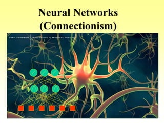
Neural Networks
(Connectionism)

2. 2
Course No.: CSC 445
Lect.: 4 h
Lab. : 2 h
Marks: 65 final
10 Y. work
25 Lab
Exam hours: 3 h
By Prof. Dr. :
Taymoor Nazmy

3. 3
Neural Networks
Textbooks:
1- Neural networks : A comprehensive foundation,
by Simon Haykin.
2- Fausett, L. : Fundamentals of Neural Networks.
Prentice Hall.

4. 4
1- Biological Neural Networks
2- BNN versus ANN
3- The McCulloch-Pitts model
4- NN components
5- Types of NN
6-Applications of NN
7- Historical notes
13- Hopfield NN
14- Radial basis function
15- Self organized map
16- Principal component
analysis PCA
Main Topics
I-Comprehensive Introduction II-Learning Algorithms
III-Some Types of NN
8- Learning process
9- Hebbian Learning
10- Perception Learning
11- Backpropagation
12- Multilayer perception,

5. 5
Reports Titles (slides)
1. The McCulloch-Pitts model
2. Applications of NN
3. Hebbian Learning
4. Perception Learning
5. Backpropagation
6. Classification using NN
7. Regression using NN
8. Hopfield NN
9. Radial basis function
10.Self organized map
11.Principal component analysis PCA
12.Learning vector quantization
13.ART NN
14.Boltzman machine
15.Reinforcement learning
3 students for each title, 10-15 slide,
max 3 group for each title, each dept.
deliver 1CD

6. 6
Introduction
• Connectionism is an approach in the fields of
artificial intelligence, cognitive science,
psychology and philosophy of mind.
• Neural networks are by far the dominant form of
connectionist model today. A lot of research
utilizing neural networks is carried out under the
more general name "connectionist".

7. 7
• Neural networks grew out of research in Artificial
Intelligence; specifically, attempts to mimic the fault-
tolerance and capacity to learn of biological neural
systems by modeling the low-level structure of the
brain .
• The main branch of Artificial Intelligence research in
the 1960s -1980s produced Expert Systems. These are
based upon a high-level model of reasoning processes .
• It became rapidly apparent that these systems, although
very useful in some domains, failed to capture certain
key aspects of human intelligence.
• In order to reproduce intelligence, it would be
necessary to build systems with a similar architecture.

8. 8
• Artificial Neural Systems are called:
– neurocomputers
– neural networks
– parallel distributed processors PDP
– connectionists systems
• Basic Philosophy
– large number of simple “neuron-like” processors
which execute global or distributed computation

9. 9
Who is concerned with NNs?
• Computer scientists want to find out about the properties of non-symbolic
information processing with neural nets and about learning systems in general.
• Statisticians use neural nets as flexible, nonlinear regression and classification models.
• Engineers of many kinds exploit the capabilities of neural networks in many areas,
such as signal processing and automatic control.
• Cognitive scientists view neural networks as a possible apparatus to describe
models of thinking and consciousness (High-level brain function).
• Neuro-physiologists use neural networks to describe and explore medium-level
brain function (e.g. memory, sensory system, motorics).
• Physicists use neural networks to model phenomena statistical mechanics and for a
lot of other tasks.
• Biologists use Neural Networks to interpret nucleotide sequences.
• Philosophers and some other people may also be interested in Neural Networks for
various reasons.

10. 10
The brain is a highly complex, non-linear, parallel information
processing system. It performs tasks like pattern recognition,
perception, motor control, many times faster than the fastest
digital computers. It characterize by;
– Robust and fault tolerant
– Flexible – can adjust to new environment by learning
– Can deal with fuzzy, probabilistic, noisy or inconsistent
information
– Is highly parallel
– Is small, compact and requires little power (10-16
J/oper/sec, comparing with 10-6 J/oper/sec for a digital
computer)
Human brain

11. 11
Man versus Machine
(hardware)
Numbers Human brain Von Neumann
computer
# elements 1010 - 1012
neurons
107 - 108
transistors
# connections /
element
104 10
switching frequency 103 Hz 109 Hz
energy / operation 10-16 Joule 10-6 Joule
power consumption 10 Watt 100 - 500 Watt
reliability of elements low reasonable
reliability of system high reasonable

12. 12
Man versus Machine
(information processing)
Features Human
Brain
Von Neumann
computer
Data representation analog digital
Memory
localization
distributed localized
Control distributed localized
Processing parallel sequential
Skill acquisition learning programming

13. 13
Super computer
Cray C90
Common House Fly
●10-9 sec transfer
●1010 ops per sec
●16 processors
●chip requires
●10-7 joules per op
●fragile
●team of maintainers
●fills a room
●10-3 sec transfer
●1011 ops per sec
●100,000 neurons
●neuron requires
●10-15 joules per op
●damage resistant
●maintains itself
●flies through a room

14. 14
Neuron structure
• Human brain consists of approximately 1011
elements called neurons.
• Communicate through a network of long
fibres called axons.
• Each of these axons splits up into a series of
smaller fibres, which communicate with other
neurons via junctions called synapses that
connect to small fibers called dendrites
attached to the main body of the neuron

15. 15
Neuron structure
• Basic computational unit is the Neuron
– Dendrites (inputs, 1 to 104 per neuron)
– Soma (cell body)
– Axon (output)
-Synapses
-excitatory
-inhibitory

16. 16
Interconnectedness
– 80,000 neurons per square mm
– 1015 connections
– Most axons extend less than
1 mm (local connections)
• Some cells in cerebral cortex may have 200,000
connections
• Total number of connections in the brain “network” is
astronomical—greater than the number of particles in
known universe

17. 17
Neuron structure
• Synapse like a one-way valve. Electrical signal is
generated by the neuron, passes down the axon, and is
received by the synapses that join onto other neurons
dendrites.
• Electrical signal causes the release of transmitter
chemicals which flow across a small gap in the synapse
(synaptic cleft).
• Chemicals can have an excitatory effect on the receiving
neuron (making it more likely to fire) or an inhibitory
effect (making it less likely to fire)
• Total inhibitory and excitatory connections to a particular
neuron are summed, if this value exceeds the neurons
threshold the neuron fires, otherwise does not fire.

18. 18
Network of neurons

19. 19
Learning in networks of neurons
• Knowledge is represented in neural networks by the strength
of the synaptic connections between neurons (hence
“connectionism”)
• Learning in neural networks is accomplished by adjusting
the synaptic strengths (aka synaptic weights, synaptic
efficacy)
• There are three primary categories of neural network
learning algorithms :
– Supervised — exemplar pairs of inputs and (known,
labeled) target outputs are used for training.
– Reinforcement — single good/bad training signal used
for training.
– Unsupervised — no training signal; self-organization
and clustering produce (and are produced by) the
“training”

20. 20
BNNs versus ANNs
An artificial neuron
A physical neuron
• From experience:
examples / training
data
• Strength of
connection between
the neurons is
stored as a weight-
value for the
specific connection.
• Learning the
• solution to a
problem = changing
the connection
weights

21. 21
Artificial Neuron
An artificial neuron
A physical neuron
• From experience:
examples / training
data
• Strength of
connection between
the neurons is stored
as a weight-value for
the specific
connection.
• Learning the solution
to a problem =
changing the
connection weights

22. 22
Idealized neurons
• To model things we have to idealize them (e.g.
atoms)
– Idealization removes complicated details that are not
essential for understanding the main principles
– Allows us to apply mathematics and to make analogies
to other, familiar systems.
– Once we understand the basic principles, its easy to add
complexity to make the model more faithful
• It is often worth understanding models that are
known to be wrong (but we mustn’t forget that
they are wrong!)
– E.g. neurons that communicate real values rather than
discrete spikes of activity.

23. 23
Neural networks abstract from
the details of real neurons
• Conductivity delays are neglected
• An output signal is either discrete (e.g., 0 or
1) or it is a real-valued number (e.g.,
between 0 and 1)
• Net input is calculated as the weighted sum
of the input signals
• Net input is transformed into an output
signal via a simple function (e.g., a
threshold function)

24. 24
What is a Neural Network?
• There is no universally accepted definition of an NN. But
perhaps most people in the field would agree that
• an NN is a network of many simple processors
(“units”), each possibly having a small amount of local
memory.
• The units are connected by communication channels
(“connections”) which usually carry numeric (as
opposed to symbolic) data, encoded by any of various
means.
• The units operate only on their local data and on the
inputs they receive via the connections.

25. 25
In present one, we introduce
= Artificial foundations of neural computation
Artificial Neural Networks
Biological foundations Artificial foundations
(Neuroscience) (Statistics, Mathematics)

26. 26
Basic Artificial Model
• Consists of simple processing elements called neurons,
units or nodes.
• Each neuron is connected to other nodes with an
associated weight (strength).
• Each neuron has a single threshold value.
• Weighted sum of all the inputs coming into the neuron is
formed and the threshold is subtracted from this value =
activation.
• Activation signal is passed through an activation function
(a.k.a. transfer function) to produce the output of the
neuron.

27. 27
The McCulloch-Pitts Model
(First Neuron Model - 1943 )
• The neuron has binary inputs (0 or 1) labelled xi
where i = 1,2, ...,n.
• These inputs have weights of +1 for excitatory
synapses and -1 for inhibitory synapses labelled
wi where i = 1,2, ...,n.
• The neuron has a threshold value T which has to
be exceeded by the weighted sum of signals if
the neuron is to fire.
• The neuron has a binary output signal denoted
by o.
• The superscript t = 0, 1, 2, ... denotes discrete
time instants.

28. 28
• The output o at a time t+1 can be defined by the
following equation:
Ot+1 = 1 if wi xi
t >= T
Ot+1 = 0 if wi xi
t < T
• i.e. output of the neuron at time t+1 is 1 if the sum
of all the inputs x at time t multiplied by their
weights w is greater than or equal to the threshold
T, and 0 if the sum of all the inputs x at time t
multiplied by their weights is less than the
threshold T.
• Simplistic, but can perform basic logic operations
NOT, OR and AND.

n
i 1

n
i 1

29. 29
Mathematical Representation
b
w1
w2
wn
x1
x2
xn
+
b
x0
f(n).
.
.
.
n
y
Inputs Weights Summation Activation Output
Inputs
Output
w2
w1
wn
.
.
…
y
1
net b
y f(net)
n
i i
i
w x



 ＋x2
xn
b
x1

30. 30
Adding biases
• A linear neuron is a more flexible model if we include a bias.
• A Bias unit can be thought of as a unit which always has an output value of 1, which is
connected to the hidden and output layer units via modifiable weights.
• It sometimes helps convergence of the weights to an acceptable solution A bias is exactly
equivalent to a weight on an extra input line that always has an activity of 1.
21 wwb
211 xx
i
i
i wxby 

1
output
bias
index over
input connections
i inputth
i th
weight on
input
x1-x2=0
x1-x2= 1
x1
x2
x1-x2= -1
bw
xwy i
m
i
i

 
0
0
OR
m

31. 31
Bias as extra input
Input
Attribute
values
weights
Summing function
Activation
function
v
Output
class
y
x1
x2
xm
w2
wm
W1
 
 )(xf
w0
x0 = +1
bw
xwy j
m
j
j

 
0
0

32. 32
Elements of the model neuron :
• Xi is the input to synapse i
• wij is the weight characterizing the synapse
from input j to neuron i
• wij is known as the weight from unit j to unit i
• wij > 0 synapse is excitatory
• wij < 0 synapse is inhibitory
• Note that Xi may be
• – external input
• – or the output of some other neuron

33. 33
• Each neuron is composed of two units. First
unit adds products of weights coefficients
and input signals.
• The second unit realize nonlinear function,
called neuron activation function. Signal x
is adder output signal, and y = f(x) is output
signal of nonlinear element.
• Signal y is also output signal of neuron.

34. 34
Neural Computation
• A single output neuron
1210202 xwxwnetinput 
Output Neuron
Input Neurons

j
jiji xwnetinput


 

otherwise0.0
0.0netinputif1.0 i
iy
20w 21w
0x 1x
2xi
j

35. 35
Computing with Neural Units
• Inputs are presented to input units
• How do we generate outputs?
• One idea
– Summed Weighted Inputs
3
1
0.3
-0.1
2.1
-1.1
Input: (3, 1, 0, -2)
Processing:
3(0.3) + 1(-0.1) + 0(2.1) + -2(-1.1)
= 0.9 + (-0.1) + 2.2
Output: 3
0
-2

36. 36
Activation Functions
• Usually, we don’t just use weighted sum directly
• Apply some function to the weighted sum before it
is used (e.g., as output)
• Call this the activation function
• Step function could be a good simulation of a
biological neuron spiking











x0
x1
)(
if
if
xf
 Is called the
threshold (T)
Step function
f(n),
f(net)
f(e)

37. 37
Activation Functions
Example: Step Function
• Let  = 3
3
1
f (3) 1
Input: (3, 1, 0, -2)
Output after passing through
step activation function:
x
f(x)
3
1
0.3
-0.1
2.1
-1.1
0
-2
X=3

38. 38
Step Function Example (2)
• Let  = 3
0.3
-0.1
2.1
-1.1
3
1
f (x) ?
Input: (0, 10, 0, 0)
Output after passing through
step activation function:
x

39. 39
Another Activation Function:
The Sigmoidal
• The math of some neural nets requires that
the activation function be continuously
differentiable
• A sigmoidal function often used to
approximate the step function
x
e
xf 


1
1
)(
 Is the
steepness
parameter

40. 40
Sigmoidal
0
0.2
0.4
0.6
0.8
1
1.2
-5
-4.4
-3.8
-3.2
-2.6
-2
-1.4
-0.8
-0.2
0.4
1
1.6
2.2
2.8
3.4
4
4.6
1/(1+exp(-x)))
1/(1+exp(-10*x)))

41. 41
Sigmoidal Example
0.3
-0.1
2.1
-1.1
f (3) 
1
1 e2x
 .998
  2

f (x) 
1
1 e2x
Input: (3, 1, 0, -2)
If an Input: (0, 10, 0, 0)
what is network output?

42. 42
n
e
nfa 


1
1
)(






00
01
)(
n
n
nfa
nnfa  )(
2
( ) n
a f n e
 
Some Activation Functions

43. 43
• Types of activation functions
• Typically, the activation function generates either
unipolar or bipolar signals.
unipolar bipolar

44. 44
Logic Functions Using Neuron model
AND
input output
00
01
10
11
0
0
0
1
y
x
1 x2
w
1 w
2
f(x1w1 + x 2w2) = y
f(0w
1
+ 0w
2
) = 0
f(0w
1
+ 1w
2
) = 0
f(1w
1
+ 0w
2
) = 0
f(1w
1
+ 1w
2
) = 1
 = 0.5
f(e) =
1, for e > 
0, for e < 
some possible values for w1 and w2
w1
w2
0.20
0.20
0.25
0.40
0.35
0.40
0.30
0.20
q
What are the possible values
For OR, NOT functions?

45. 45
What about XOR
input output
00
01
10
11
0
1
1
0
y
x1 x2
w
1 w
2
f(x1w1 + x2w2) = y
f(0w
1
+ 0w
2
) = 0
f(0w
1
+ 1w
2
) = 1
f(1w1 + 0w2) = 1
f(1w1 + 1w2) = 0
 = 0.5
f(e) = 1, for e > 
0, for e < 
some possible values for w1 and w2
w1
w2
q
? ?

46. 46
• If a threshold function is a
linearly separable function.
This implies that the
function is capable of
assigning all inputs to two
categories ( basically a
classifier ).
If  = w0 + w1x1 + w2x2 ,
• This equation can be viewed
as an equation of a line.
Depending on the values of
the weights, this line will
separate the four possible
inputs into two categories.
• •
• •
x2
x1
w0 = -1
w1 = 1
w2 = 1
w0 = 1
w1 = 1
w2 = 1
w0 = 1
w1 = -1
w2 = 1
A B
CD
Linearly Separable Function

47. 47
Linear Separability of logic
functions
• Boolean AND, OR and XOR
Input AND OR XOR
0 0 0 0 0
1 0 0 1 1
0 1 0 1 1
1 1 1 1 0
• Partitioning Problem
Space
1,1
1,00,0
0,1 1,1
1,00,0
0,1
1,1
1,00,0
0,1 1,1
1,00,0
0,1
OR
XOR
AND

48. 48

49. 49
Slope= (6-0)/(0-6)= -1
X2 intersection=6
(0,6)
(6,0)

50. 50

51. 51

52. 52

53. 53

54. 54

55. 55
XOR
input output
00
01
10
11
0
1
1
0
f(e) = 1, for e > 
0, for e  

f(w1, w2, w3, w4, w5 , w6)
a possible set of values for ws
(w1, w2, w3, w4, w5 , w6)
(0.6,-0.6,-0.7,0.8,1,1)
w1 w4w3
w2
w5 w6
 = 0.5 for all units

56. 56
Another solution for XOR
x1
x2
-1
+1
+1
+1
+1
-1
-1
-1
0.1

57. 57
Another Example
• A two weight layer, feedforward network
• Two inputs, one output, one ‘hidden’ unit
0.5
-0.5
Input: (3, 1)
x
e
xf 


1
1
)(
0.75
What is the output?

58. 58
Types of decision regions
022110  xwxww
022110  xwxww
x1
1
x2
Convex
region
L1 L2
L3L4
-3.5
Network
with a single
node
One-hidden layer network that
realizes the convex region: each
hidden node realizes one of the
lines bounding the convex region
1
1
1
1
1
x1
x2
1
w0
w1
w2
Each neuron in the second layer presents a hyperplane.

59. 59
Structure
Types of
Decision Regions
Exclusive-OR
Problem
Classes with
Meshed regions
Most General
Region Shapes
Single-Layer
Two-Layer
Three-Layer
Half Plane
Bounded By
Hyperplane
Convex Open
Or
Closed Regions
Arbitrary
(Complexity
Limited by No.
of Nodes)
A
AB
B
A
AB
B
A
AB
B
B
A
B
A
B
A
Different non linearly separable
problems

60. 60
Basic Neural Network & Its Elements
Input
Neurons
Hidden
Neurons
Output
Neurons
Bias Neurons

61. 61
Hidden Units
• Hidden units are a layer of nodes that are situated
between the input nodes and the output nodes.
• Hidden units allow a network to learn non-linear
functions.
• Too few hidden layer units, the network may fail to
train correctly
• Too many and as well as increased training times,
the network may fail to generalise correctly, i.e. it
may become too specific on the patterns it has been
trained on, and unable to respond correctly to novel
patterns..

62. 62
Number of hidden units
• There are no concrete guidelines for the determination of the
number of hidden layer units.
• Often obtained by experimentation, or by using optimizing
techniques such as genetic algorithms.
• It is possible to remove hidden units that are are not
participating in the learning process by examining the weight
values on the hidden units periodically as the network trains,
on some units the weight values change very little, and these
units may be removed from the network.

63. 63
Example: Mapping from input to
output
0.2 -0.5 0.8
0.5 1.0 -0.1 0.2
-0.9 0.2 -0.1 0.7
Input pattern: <0.5, 1.0,-0.1,0.2>
input layer
hidden layer
Output pattern: <-0.9, 0.2,-0.1,0.7>
output layer
feed-forward
processing

64. 64
Vector Notation
• At times useful to represent weights and
activations using vector and matrix
notations
W1,1
W1,2
W1,3
W1,4
1,2x
1,3x
1,4x
2,1x
1,1x
Weight (scalar) from unit j
in left layer to unit i in
right layer
jiW ,
Activation value of unit k in
layer l; layers increase in
number from left to right
lkx ,
(Layer 1, unit i for W, and unit k for a)
(Layer 2, unit j for W, and k for a)

65. 65
Notation for Weighted Sums
2,1x )( 1,44,11,33,11,22,11,11,1 xWxWxWxWf 
1,4x
W1,1
W1,2
W1,3
W1,4
1,2x
1,3x 2,1x
1,1x
)( 1 ,,1,  
n
i lkjilk xWfx
Generalizing

66. 66
Can Also Use Vector Notation
iW Row vector of incoming weights for unit i
ix Column vector of activation values of units
connected to unit i
(Assuming that the layer for unit i is specified in the context)

67. 67
Weight Matrices
x1
x2
x3
i 1
3
xi w1i
i 1
3
xi w2 i
i 1
3
xi w3i
i 1
3
xi w4 i
w11
w41
w13
w43
XW

68. 68
Example
 4,13,12,11,11 WWWWW 
 













1,4
1,3
1,2
1,1
4,13,12,11,111
a
a
a
a
WWWWaW













4
3
2
1
1
a
a
a
a
a
Recall: multiplying a
n*r with a r*m matrix
produces an n*m matrix,
C, where each element in
that n*m matrix Ci,j is
produced as the scalar
product of row i of the
left and column j of the
right
1,4a
W1,1
W1,2
W1,3
W1,4
1,2a
1,3a 2,1a
1,1a
If the input for a NN is given by a vector a ,and its weight by W
1,44,11,33,11,22,11,11,1 aWaWaWaW 

69. 69
Notation
ia The vector of activation values of layer to
“left”; an r*1 column vector (same as before)
iaW
n*1 column vector;
summed weights for
“right” layer
)( iaWf n*1 - New activation values for
“right” layer
Function f is now taken as applying to
elements of a vector

70. 70
Example
)
75.
4.0
23
02
11.1
34
0.31
( 






















f
Updating hidden
layer activation
values
)
1
3
3
2
1.
6.3310
56471.
4.1322
(


























f
Updating output
activation values
Draw the architecture (units and arcs representing
weights) of the connectionist model presented by
the following function.
)( iaWf
5x2
2x1
3x5
5x1

71. 71
Answer
• 2 input units
• 5 hidden layer units
• 3 output units
• Fully connected, feedforward network

72. 72
The main characteristics of NN
• Architecture: the pattern of nodes and
connections between them
• Learning algorithm, or training method:
method for determining weights of the
connections
• Activation function: function that
produces an output based on the input
values received by node

73. 73
Taxonomy of neural networks
Feedforward Recurrent
(Kohonen) (MLP, RBF)
Unsupervised Supervised
(ART) (Elman, Jordan,
Hopfield)
Unsupervised Supervised

74. 74
Types of connectivity
1-Feedforward networks
– The neurons are arranged in separate
layers
– There is no connection between the
neurons in the same layer
– The neurons in one layer receive inputs
from the previous layer
– The neurons in one layer delivers its
output to the next layer
– The connections are unidirectional
– (Hierarchical)
2-Recurrent networks
Some connections are present from a layer
to the previous layers More biologically
realistic.
• Feedforward + feedback = recurrent
hidden units
output units
input units

75. 75
Types of connectivity
• 3-Associative networks
– There is no hierarchical arrangement
– The connections can be bidirectional

76. 76
• Spiking (or pulsed) neural networks (SNNs) are models
which explicitly take into account the timing of inputs. The
network input and output are usually represented as series
of spikes (delta function or more complex shapes). SNNs
have an advantage of being able to continuously process
information. They are often implemented as recurrent
networks.
• Networks of spiking neurons - (e.g. PCNN pulse coupled
neural network, can be used for image processing
purposes as well as pattern recognition, and it shows a
unique feature which is a signature that is invariant
with respect to scaling, transition, and rotation).
Other Important NN Models
Spiking neural networks

77. 77
• Biological studies showed that the human
brain functions not as one single massive
network, but as a collection of small
networks.
• This realization gave birth to the concept of
Modular neural networks, in which several
small networks cooperate or compete to
solve problems.
Modular neural networks

78. 78
Developing Neural Networks
Step 1:
• collect data, and preprocess it,
Step 2:
• separate data into training and test sets,
usually random separation
• ensure that application is amenable to a NN
approach

79. 79
Developing Neural Networks
Step 3:
• define a network structure
Step 4:
• select a learning algorithm
Step 5:
• set parameter values
Step 6:
• transform Data to Network Inputs
• data must be NUMERIC, may need to preprocess the
data, e.g., normalize values for a range of 0 to 1

80. 80
Developing Neural Networks
Step 7:
• start training
• determine and revise weights, check points
Step 8:
• stop and test: iterative process
Step 9:
• implementation
• stable weights obtained
• begin using the system

81. 81
Artificial
Neural
Network
Development
Process
Implementation
Stop and Test
Start Training
Transform Data into Network Inputs
Set Parameter Values
Select a Learning Algorithm
Define a Network Structure
Separate into Training and Test Sets
Collect Data
Reset
Reset
Select Another
Algorithm
Refine
Structure
Get More,
Better Data

82. 82
Data Collection and Preparation
• Collect data and separate into a training set and
a test set
• Use training cases to adjust the weights
• Use test cases for network validation

83. 83
Types of pre-processing
1. Linear transformations
e.g input normalization
2. Dimensionality reduction
lose irrelevant info and retain important features
3. Feature extraction
use a combination of input variables: can incorporate 1, 2 and 3
4. Feature selection
decide which features to use

84. 84
Dimensionality Reduction
Clearly losing some information but this can be helpful
due to curse of dimensionality
Need some way of deciding what dimensions to keep
1. Random choice
2. Principal components analysis (PCA)
3. Independent components analysis (ICA)
4. Self-organized maps (SOM)

85. 85
Neural network input normalization
Real input data values are standardized (scaled),
normalized so that they all have ranges from 0 – 1.
valueattributepossiblelargesttheisuemaximumVal
attributefor thevaluepossiblesmallesttheisueminimumVal
convertedbetovaluetheislueoriginalVa
rangeinterval[0,1]theinfallingvaluecomputedtheisnewValue
where
ueminimumValuemaximumVal
ueminimumVallueoriginalVa
newValue




86. 86
The basic Learning process : Three Tasks
1. Compute Outputs
2. Compare Outputs with Desired Targets
3. Adjust Weights and Repeat the Process.
• Set the weights by either rules or randomly
• Set Delta = Error = actual output minus desired output
for a given set of inputs
• Objective is to Minimize the Delta (Error)
• Change the weights to reduce the Delta

87. 87
Set the parameters values
• Determine several parameters
– Learning rate (high or low)
– Threshold value for the form of the output
– Initial weight values
– Other parameters
• Choose the network's structure (nodes and layers)
• Select initial conditions
• Transform training and test data to the required format
Testing
• Test the network after training
• Examine network performance: measure the network’s
classification ability
• Not necessarily 100% accurate

88. 88
Overtraining (overfitting)
• It is possible to train a network too much, where the
network becomes very good at classifying the training
set, but poor at classifying the test set that it has not
encountered before, i.e. it is not generalising well.
• Early stopping
The only way to avoid this is to periodically present the test set
to the network, and record the error whilst storing the weights
at the same time, in this way an optimum set of weights giving
the minimum error on the test set can be found. Some neural
network packages do this for you in a way that is hidden from
the user.

89. 89
overtraining

90. 90
Types of Problems Solved by NN
• Classification: determine to which of a
discrete number of classes a given input case
belongs
• Regression: predict the value of a (usually)
continuous variable
• Times series- you wish to predict the value of
variables from earlier values of the same or other
variables

91. 91
Types of NNs
• Here are some well-known kinds of NNs:
Supervised
I- Feedforward
• Linear
– Hebbian - Hebb (1949), Fausett (1994)
– Perceptron - Rosenblatt (1958), Minsky and Papert
(1969/1988), Fausett (1994)
– Adaline - Widrow and Hoff (1960), Fausett (1994)
– Higher Order - Bishop (1995)
– Functional Link - Pao (1989)
• MLP: Multilayer perceptron - Bishop (1995), Reed and
Marks (1999), Fausett (1994)
– Backprop - Rumelhart, Hinton, and Williams (1986)
– Cascade Correlation - Fahlman and Lebiere (1990),
Fausett (1994)
– Quickprop - Fahlman (1989)
– RPROP - Riedmiller and Braun (1993)

92. 92
• RBF networks - Bishop (1995), Moody and Darken
(1989), Orr (1996)
– OLS: Orthogonal Least Squares - Chen, Cowan
and Grant (1991)
• CMAC: Cerebellar Model Articulation Controller -
Albus (1975), Brown and Harris (1994)
• Classification only
– LVQ: Learning Vector Quantization - Kohonen
(1988), Fausett (1994)
– PNN: Probabilistic Neural Network - Specht
(1990), Masters (1993), Hand (1982), Fausett
(1994)
• Regression only
– GNN: General Regression Neural Network -
Specht (1991), Nadaraya (1964), Watson (1964)

93. 93
• II-Feedback
• - Hertz, Krogh, and Palmer (1991), Medsker and Jain (2000)
• BAM: Bidirectional Associative Memory - Kosko (1992), Fausett
(1994)
• Boltzman Machine - Ackley et al. (1985), Fausett (1994)
• Recurrent time series
– Backpropagation through time - Werbos (1990)
– Elman - Elman (1990)
– FIR: Finite Impulse Response - Wan (1990)
– Jordan - Jordan (1986)
– Real-time recurrent network - Williams and Zipser (1989)
– Recurrent backpropagation - Pineda (1989), Fausett (1994)
– TDNN: Time Delay NN - Lang, Waibel and Hinton (1990)

94. 94
• III-Competitive
• ARTMAP - Carpenter, Grossberg and Reynolds (1991)
• Fuzzy ARTMAP - Carpenter, Grossberg, Markuzon,
Reynolds and Rosen (1992), Kasuba (1993)
• Gaussian ARTMAP - Williamson (1995)
• Counterpropagation - Hecht-Nielsen (1987; 1988;
1990), Fausett (1994)
• Neocognitron - Fukushima, Miyake, and Ito (1983),
Fukushima, (1988), Fausett (1994)

95. 95
2-Unsupervised
I- Competitive
– Vector Quantization
• Grossberg - Grossberg (1976)
• Kohonen - Kohonen (1984)
• Conscience - Desieno (1988)
– Self-Organizing Map
• Kohonen - Kohonen (1995), Fausett (1994)
• GTM: - Bishop, Svensén and Williams (1997)
• Local Linear - Mulier and Cherkassky (1995)

96. 96
• Adaptive resonance theory
• ART 1 - Carpenter and Grossberg (1987a), Moore (1988),
Fausett (1994)
• ART 2 - Carpenter and Grossberg (1987b), Fausett
(1994)
• ART 2-A - Carpenter, Grossberg and Rosen (1991a)
• ART 3 - Carpenter and Grossberg (1990)
• Fuzzy ART - Carpenter, Grossberg and Rosen (1991b)
• DCL: Differential Competitive Learning - Kosko (1992)

97. 97
• II- Dimension Reduction
• Hebbian - Hebb (1949), Fausett (1994)
• Oja - Oja (1989)
• Sanger - Sanger (1989)
• Differential Hebbian - Kosko (1992)
III-Autoassociation
• Linear autoassociator - Anderson et al. (1977), Fausett
(1994)
• BSB: Brain State in a Box - Anderson et al. (1977), Fausett
(1994)
• Hopfield - Hopfield (1982), Fausett (1994)

98. 98
Advantages of ANNs
• Generalization :using responses to prior input
patterns to determine the response to a novel input
• Inherent massively parallel
• Able to learn any complex non-linear mapping
• Learning instead of programming
• Robust
– Can deal with incomplete and/or noisy data
• Fault-tolerant
– Still works when part of the net fails

99. 99
Disadvantages of ANNs
• Difficult to design
• The are no clear design rules for arbitrary applications
• Learning process can be very time consuming
• Can overfit the training data, becoming useless for generalization
• Difficult to assess internal operation
– It is difficult to find out whether, and if so what tasks are
performed by different parts of the net
• Unpredictable
– It is difficult to estimate future network performance based on
current (or training) behavior

100. 100
ANN Application Areas
• Classification
• Clustering
• Associative memory
• Control
• Function approximation (Modelling)

101. 101
Applications for ANN Classifiers
• Pattern recognition
– Industrial inspection
– Fault diagnosis
– Image recognition
– Target recognition
– Speech recognition
– Natural language processing
• Character recognition
– Handwriting recognition
– Automatic text-to-speech conversion

102. 102
ANN Clustering Applications
• Natural language processing
– Document clustering
– Document retrieval
– Automatic query
• Image segmentation
• Data mining
– Data set partitioning
– Detection of emerging clusters
• Fuzzy partitioning
• Condition-action association

103. 103
ANN Control Applications
• Non-linear process control
– Chemical reaction control
– Industrial process control
– Water treatment
– Intensive care of patients
• Servo control
– Robot manipulators
– Autonomous vehicles
– Automotive control
• Dynamic system control
– Helicopter flight control
– Underwater robot control

104. 104
ANN Modelling Applications
• Modelling of highly nonlinear industrial
processes
• Financial market prediction
• Weather forecasts
• River flow prediction
• Fault/breakage prediction
• Monitoring of critically ill patients

105. 105
History of Neural Networks
BNN:
• 1887 - Sherrington: Synaptic interconnection
suggested
• 1920's - discovered that neurons communicate
via chemical impulses called neurotransmitters.
• 1930's - research on the chemical processes that
produce the electrical impulses.

106. 106
History
ANN:
• Early stages
– 1943 McCulloch-Pitts: neuron as comp. elem.
– 1949 Hebb: learning rule
– 1958 Rosenblatt: perceptron
– 1960 Widrow-Hoff: least mean square algorithm
• Recession
– 1969 Minsky-Papert: limitations perceptron model
• Revival
– 1982 Hopfield: recurrent network model
– 1982 Kohonen: self-organizing maps
– 1986 Rumelhart et. al.: backpropagation

107. 107
Some details of neural networks History
• Bernard Widrow and Ted Hoff, in 1960, introduced the Least-
Mean-Squares algorithm (delta-rule or Widrow-Hoff rule)
and used it to train ADALINE (ADAptive LINear Elements
or ADAptive LInear NEurons)
• Marvin Minsky and Seymour Papert, in 1969, published
Perceptrons, in which they mathematically proved that single-
layer perceptrons were only able to distinguish linearly
separable classes of patterns
– While true, they also (mistakenly) speculated that an
extension to multiple layers would lose the “virtue” of the
perceptron’s simplicity and be otherwise “sterile”
– As a result of Minsky & Papert’s Perceptrons, research in
neural networks was effectively abandoned in the 1970s
and early 1980s

108. 108
History of neural networks
• Shun-ichi Amari, in 1967, and Christoph von der
Malsburgh, in 1973, published ANN models of self-
organizing maps, but the work was largely ignored
• Paul Werbos, in his 1974 PhD thesis, first
demonstrated a method for training multi-layer
perceptrons, essentially identical to Backprop but the
work was largely ignored
• Stephen Grossberg and Gail Carpenter, in 1980,
established a new principle of self-organization called
Adaptive Resonance Theory (ART), largely ignored at
the time
• John Hopfield, in 1982, described a class of recurrent
networks as an associative memory using statistical
mechanics; now known as Hopfield networks, this
work and Backprop are considered most responsible
for the rebirth of neural networks

109. 109
History of neural networks
• Teuvo Kohonen, in 1982, introduced SOM algorithms for
Self-Organized Maps, that continue to be explored and
extended today
• David Parker, in 1982, published an algorithm similar to
Backprop, which was ignored
• Kirkpatrick, Gelatt and Vecchi, in 1983, introduced
Simulated Annealing for solving combinatorial optimization
problems
• Barto, Sutton, and Anderson in 1983 popularized
reinforcement learning (it had been addressed briefly by
Minsky in his 1954 PhD dissertation)
• Yann LeCun, in 1985, published an algorithm similar to
Backprop, which was again ignored

110. 110
END of the slides