Download to read offline


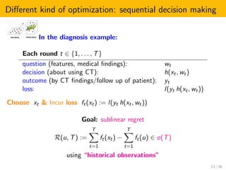


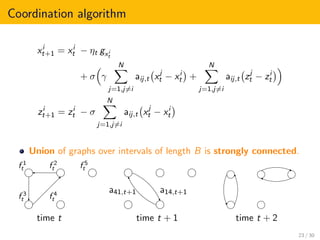
![Our contributions (informally)
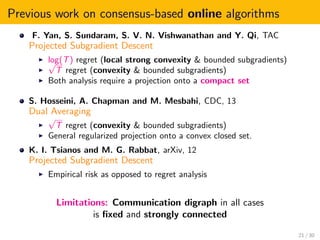
time-varying communication digraphs under B-joint connectivity &
weight-balanced
unconstrained optimization (no projection step onto a bounded set)
log T regret (local strong convexity & bounded subgradients)
√
T regret (convexity & β-centrality with β ∈ (0, 1] & bounded
subgradients)
22 / 30](https://image.slidesharecdn.com/c8366a48-50a3-422b-bf2a-dc755610443c-160415140434/85/slides_online_optimization_david_mateos-33-320.jpg)
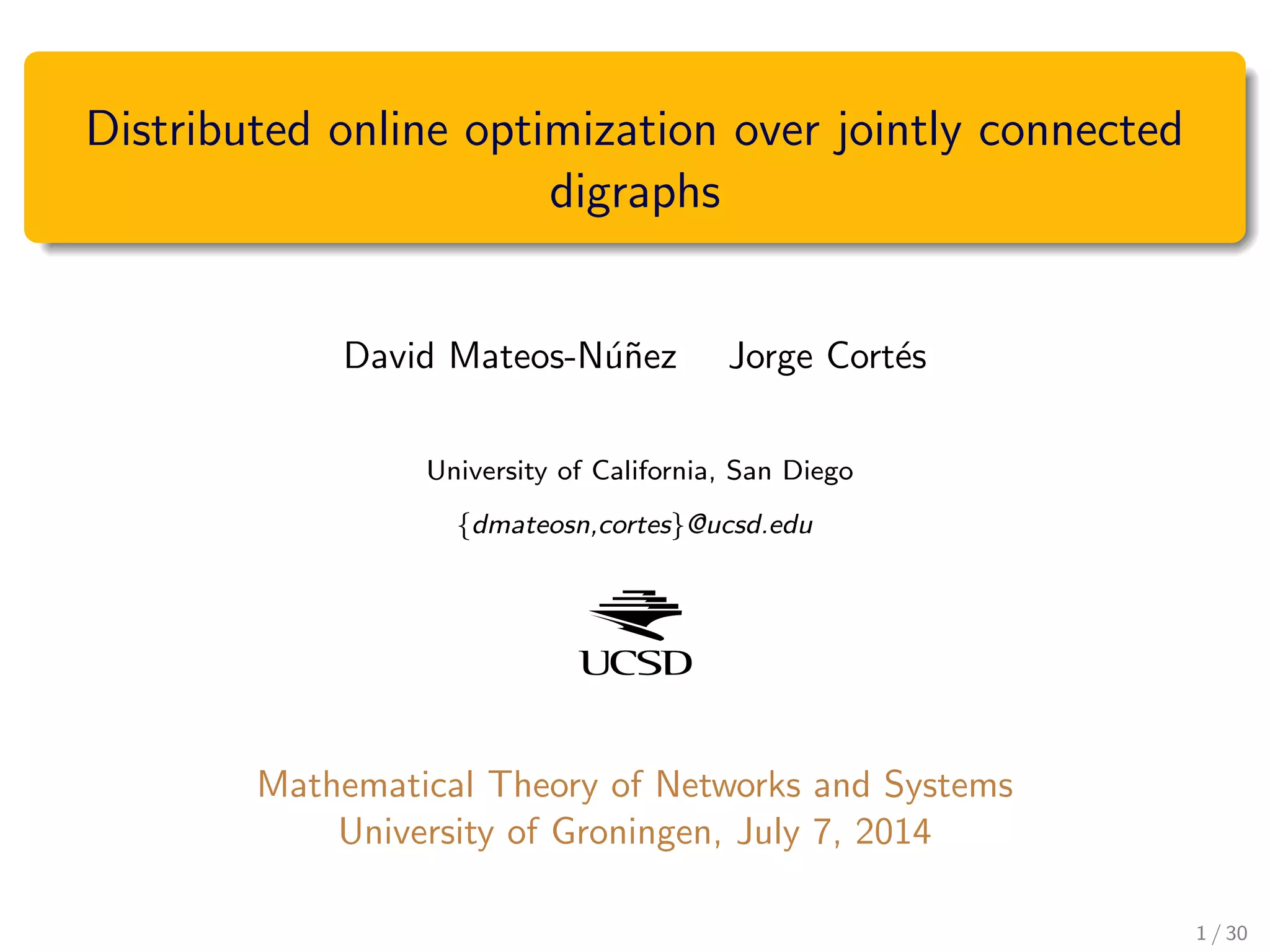
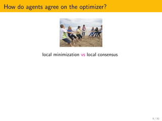
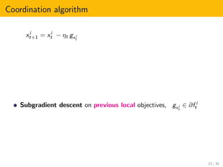
![Our contributions (informally)
time-varying communication digraphs under B-joint connectivity &
weight-balanced
unconstrained optimization (no projection step onto a bounded set)
log T regret (local strong convexity & bounded subgradients)
√
T regret (convexity & β-centrality with β ∈ (0, 1] & bounded
subgradients)
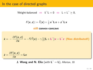
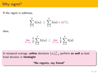
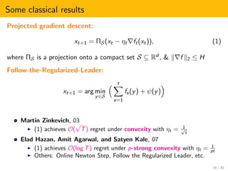
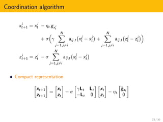
x∗
x
−ξx
f i
t is β-central in Z ⊆ Rd X∗,
where X∗ = x∗ : 0 ∈ ∂f i
t (x∗) ,
if ∀x ∈ Z, ∃x∗ ∈ X∗ such that
−ξx (x∗ − x)
ξx 2 x∗ − x 2
≥ β,
for each ξx ∈ ∂f i
t (x).
22 / 30](https://image.slidesharecdn.com/c8366a48-50a3-422b-bf2a-dc755610443c-160415140434/85/slides_online_optimization_david_mateos-34-320.jpg)
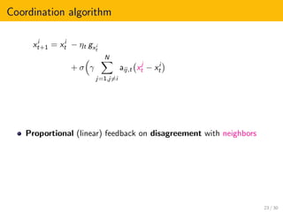
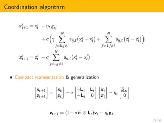
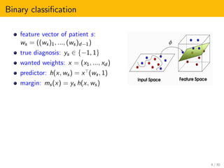
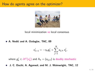
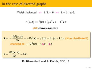
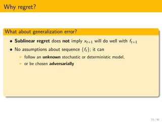
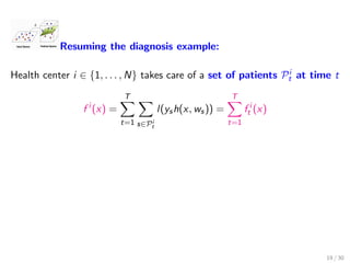
![Theorem (DMN-JC)
Assume that
{f 1
t , ..., f N
t }T
t=1 are convex functions in Rd
with H-bounded subgradient sets,
nonempty and uniformly bounded sets of minimizers, and
p-strongly convex in a suff. large neighborhood of their minimizers
The sequence of weight-balanced communication digraphs is
nondegenerate, and
B-jointly-connected
E ∈ RK×K is diagonalizable with positive real eigenvalues
Substituting strong convexity by β-centrality, for β ∈ (0, 1],
Rj
(u, T) ≤ C u 2
2
√
T,
for any j ∈ {1, . . . , N} and u ∈ Rd
24 / 30](https://image.slidesharecdn.com/c8366a48-50a3-422b-bf2a-dc755610443c-160415140434/85/slides_online_optimization_david_mateos-42-320.jpg)

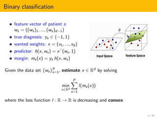
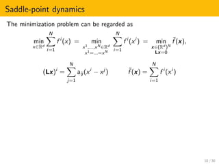
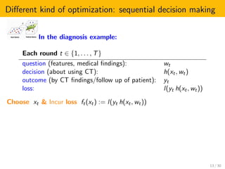
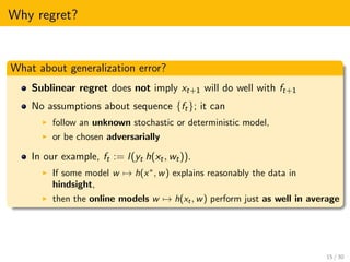
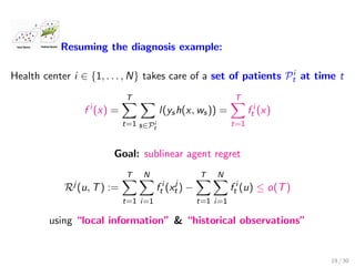
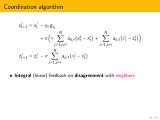
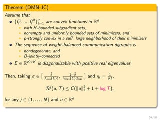
![Outline of the proof
Analysis of network regret
RN (u, T) :=
T
t=1
N
i=1
f i
t (xi
t ) −
T
t=1
N
i=1
f i
t (u)
ISS with respect to agreement
ˆLKvt 2 ≤ CI v1 2 1 −
˜δ
4N2
t−1
B
+ CU max
1≤s≤t−1
us 2,
Agent regret bound in terms of {ηt}t≥1 and initial conditions
Boundedness of online estimates under β-centrality (β ∈ (0, 1] )
Doubling trick to obtain O(
√
T) agent regret
Local strong convexity ⇒ β-centrality
ηt = 1
p t to obtain O(log T) agent regret
27 / 30](https://image.slidesharecdn.com/c8366a48-50a3-422b-bf2a-dc755610443c-160415140434/85/slides_online_optimization_david_mateos-45-320.jpg)


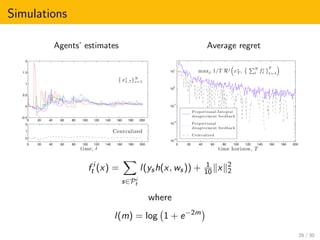
This document presents an overview of distributed online optimization over jointly connected digraphs. It discusses combining distributed convex optimization and online convex optimization frameworks. Specifically, it proposes a coordination algorithm for distributed online optimization over time-varying communication digraphs that are weight-balanced and jointly connected. The algorithm achieves sublinear regret bounds of O(sqrt(T)) under convexity and O(log(T)) under local strong convexity, using only local information and historical observations. This is an improvement over previous work that required fixed strongly connected digraphs or projection onto bounded sets.