This dissertation proposes and analyzes distributed algorithms for solving convex optimization problems in networked systems. Specifically, it considers algorithms for distributed convex optimization that are robust to noise, distributed online convex optimization over time-varying graphs, distributed saddle-point subgradient methods with consensus constraints, and distributed nuclear norm regularization for multi-task learning. It also studies stability properties of stochastic differential equations with persistent noise. The analysis establishes convergence and performance guarantees for the distributed optimization algorithms and characterizes different notions of stability for stochastic systems.

1. UNIVERSITY OF CALIFORNIA, SAN DIEGO
Distributed Algorithms for Convex Optimization:
noisy channels, online computation, nuclear norm regularization,
and separable constraints
A dissertation submitted in partial satisfaction of the
requirements for the degree
Doctor of Philosophy
in
Engineering Sciences (Mechanical Engineering)
by
David Mateos-Núñez
Committee in charge:
Professor Jorge Cortés, Chair
Professor Philip E. Gill
Professor Tara Javidi
Professor Miroslav Krstić
Professor Maurício de Oliveira
2016

2. Copyright
David Mateos-Núñez, 2016
All rights reserved.

3. The dissertation of David Mateos-Núñez is approved, and
it is acceptable in quality and form for publication on
microfilm and electronically:
Chair
University of California, San Diego
2016
iii

4. DEDICATION
To my parents,
María Luz Núñez Díaz and Carlos Mateos Mateos
iv

5. TABLE OF CONTENTS
Signature Page . . . . . . . . . . . . . . . . . . . . . . . . . . . . . . . . . . iii
Dedication . . . . . . . . . . . . . . . . . . . . . . . . . . . . . . . . . . . . . iv
Table of Contents . . . . . . . . . . . . . . . . . . . . . . . . . . . . . . . . . v
List of Figures . . . . . . . . . . . . . . . . . . . . . . . . . . . . . . . . . . viii
List of Tables . . . . . . . . . . . . . . . . . . . . . . . . . . . . . . . . . . . ix
Preface . . . . . . . . . . . . . . . . . . . . . . . . . . . . . . . . . . . . . . x
Acknowledgements . . . . . . . . . . . . . . . . . . . . . . . . . . . . . . . . xii
Vita . . . . . . . . . . . . . . . . . . . . . . . . . . . . . . . . . . . . . . . . xxvi
Abstract of the Dissertation . . . . . . . . . . . . . . . . . . . . . . . . . . . xxviii
Chapter 1 Introduction . . . . . . . . . . . . . . . . . . . . . . . . . . . . 1
1.1 Problems considered . . . . . . . . . . . . . . . . . . . . 3
1.2 Literature review . . . . . . . . . . . . . . . . . . . . . . 9
1.2.1 Distributed optimization . . . . . . . . . . . . . . 9
1.2.2 Distributed online optimization . . . . . . . . . . 14
1.2.3 Nuclear norm regularization . . . . . . . . . . . . 15
1.2.4 Stability of stochastic differential equations . . . . 16
1.3 Contributions . . . . . . . . . . . . . . . . . . . . . . . . 18
1.3.1 Noise-to-state exponentially stable distributed con-
vex optimization on weight-balanced digraphs . . 19
1.3.2 Distributed online convex optimization over jointly
connected digraphs . . . . . . . . . . . . . . . . . 20
1.3.3 Distributed saddle-point subgradient algorithms
with Laplacian averaging . . . . . . . . . . . . . . 21
1.3.4 Distributed optimization for multi-task learning
via nuclear-norm approximation . . . . . . . . . . 23
1.3.5 pth moment noise-to-state stability of stochastic
differential equations with persistent noise . . . . 24
1.4 Organization . . . . . . . . . . . . . . . . . . . . . . . . . 25
Chapter 2 Preliminaries . . . . . . . . . . . . . . . . . . . . . . . . . . . 27
2.1 Notational conventions . . . . . . . . . . . . . . . . . . . 27
2.1.1 Seminorms . . . . . . . . . . . . . . . . . . . . . . 29
2.1.2 Matrix analysis . . . . . . . . . . . . . . . . . . . 29
v

6. 2.1.3 Matrix norms . . . . . . . . . . . . . . . . . . . . 30
2.2 Convex functions . . . . . . . . . . . . . . . . . . . . . . 31
2.2.1 Comparison functions . . . . . . . . . . . . . . . . 32
2.3 Optimization . . . . . . . . . . . . . . . . . . . . . . . . 33
2.4 Variational characterizations of the nuclear norm . . . . . 34
2.5 Graph theory . . . . . . . . . . . . . . . . . . . . . . . . 36
2.6 Stochastic differential equations . . . . . . . . . . . . . . 37
Chapter 3 Noise-to-state exponentially stable distributed convex optimiza-
tion . . . . . . . . . . . . . . . . . . . . . . . . . . . . . . . . . 41
3.1 Network model and problem statement . . . . . . . . . . 42
3.2 Robust distributed optimization . . . . . . . . . . . . . . 43
3.3 Algorithm properties and stability analysis . . . . . . . . 53
3.3.1 Equilibrium points . . . . . . . . . . . . . . . . . 54
3.3.2 Co-coercivity properties of the dynamics . . . . . 55
3.3.3 Global existence and uniqueness of solutions . . . 61
3.3.4 NSS Lyapunov function . . . . . . . . . . . . . . . 62
3.3.5 Completing the proof of the main result . . . . . 73
3.4 Discussion . . . . . . . . . . . . . . . . . . . . . . . . . . 74
Chapter 4 Distributed online convex optimization over jointly connected
digraphs . . . . . . . . . . . . . . . . . . . . . . . . . . . . . . 76
4.1 Problem statement . . . . . . . . . . . . . . . . . . . . . 77
4.2 Dynamics for distributed online optimization . . . . . . . 79
4.3 Regret analysis . . . . . . . . . . . . . . . . . . . . . . . 83
4.3.1 Bounds on network and agent regret . . . . . . . 83
4.3.2 Bound on cumulative disagreement . . . . . . . . 87
4.3.3 Uniform bound on the trajectories . . . . . . . . . 96
4.4 Logarithmic and square-root agent regret . . . . . . . . . 105
4.5 Simulation: application to medical diagnosis . . . . . . . 110
4.6 Discussion . . . . . . . . . . . . . . . . . . . . . . . . . . 113
Chapter 5 Distributed saddle-point subgradient algorithms with Laplacian
averaging . . . . . . . . . . . . . . . . . . . . . . . . . . . . . 117
5.1 Distributed algorithms for saddle-point problems under
agreement constraints . . . . . . . . . . . . . . . . . . . . 118
5.1.1 Optimization problems with separable constraints 119
5.1.2 Saddle-point dynamics with Laplacian averaging . 121
5.2 Convergence analysis . . . . . . . . . . . . . . . . . . . . 123
5.2.1 Saddle-point evaluation error in terms of the dis-
agreement . . . . . . . . . . . . . . . . . . . . . . 124
5.2.2 Bounding the cumulative disagreement . . . . . . 129
vi

7. 5.2.3 Convergence of saddle-point subgradient dynamics
with Laplacian averaging . . . . . . . . . . . . . . 130
5.3 Applications to distributed constrained convex optimization136
5.3.1 Distributed strategy to bound the optimal dual set 141
5.4 Simulation example . . . . . . . . . . . . . . . . . . . . . 146
5.5 Discussion . . . . . . . . . . . . . . . . . . . . . . . . . . 149
Chapter 6 Distributed optimization for multi-task learning via nuclear-
norm approximation . . . . . . . . . . . . . . . . . . . . . . . 152
6.1 Optimization with nuclear norm regularization . . . . . . 153
6.1.1 Multi-task feature learning . . . . . . . . . . . . . 153
6.1.2 Matrix completion for recommender systems . . . 154
6.1.3 A case for distributed optimization . . . . . . . . 154
6.2 Distributed coordination algorithms . . . . . . . . . . . . 156
6.2.1 Nuclear norm approximate regularization . . . . . 156
6.2.2 Separable saddle-point formulation . . . . . . . . 161
6.3 Convergence analysis . . . . . . . . . . . . . . . . . . . . 168
6.4 Simulation example . . . . . . . . . . . . . . . . . . . . . 172
6.5 Discussion . . . . . . . . . . . . . . . . . . . . . . . . . . 173
Chapter 7 pth moment noise-to-state stability of stochastic differential
equations with persistent noise . . . . . . . . . . . . . . . . . . 175
7.1 Basic notions . . . . . . . . . . . . . . . . . . . . . . . . 176
7.1.1 Brownian motion . . . . . . . . . . . . . . . . . . 176
7.1.2 Stochastic differential equations . . . . . . . . . . 178
7.2 Noise-to-state stability via noise-dissipative Lyapunov
functions . . . . . . . . . . . . . . . . . . . . . . . . . . . 180
7.3 Refinements of the notion of proper functions . . . . . . 193
7.3.1 Proper functions and equivalence relations . . . . 194
7.3.2 Characterization of proper functions with respect
to each other . . . . . . . . . . . . . . . . . . . . 198
7.3.3 Application to noise-to-state stability . . . . . . . 207
7.4 Discussion . . . . . . . . . . . . . . . . . . . . . . . . . . 210
Chapter 8 Conclusions . . . . . . . . . . . . . . . . . . . . . . . . . . . . 212
8.1 Future directions . . . . . . . . . . . . . . . . . . . . . . 214
Chapter 9 Epilogue . . . . . . . . . . . . . . . . . . . . . . . . . . . . . . 216
Appendix A Auxiliary results . . . . . . . . . . . . . . . . . . . . . . . . . . 218
Appendix of Chapter 3 . . . . . . . . . . . . . . . . . . . . . . 218
Appendix of Chapter 7 . . . . . . . . . . . . . . . . . . . . . . 219
Bibliography . . . . . . . . . . . . . . . . . . . . . . . . . . . . . . . . . . . 222
vii

8. LIST OF FIGURES
Figure 3.1: Simulation example of our distributed continuous-time algo-
rithm (3.5) under persistent noise. . . . . . . . . . . . . . . . . 49
Figure 4.1: Visual aid in two dimensions for the proof of Lemmas 3.19 and 3.20. 98
Figure 4.2: The communication topology in our simulation example corre-
sponds to the periodic repetition of the displayed sequence of
weight-balanced digraphs. . . . . . . . . . . . . . . . . . . . . . 113
Figure 4.3: Simulated temporal average regret of the online gradient de-
scent algorithms with proportional and proportional-integral
disagreement feedback. . . . . . . . . . . . . . . . . . . . . . . . 115
Figure 4.4: Agents’ estimates for our online gradient descent algorithm with
proportional-integral disagreement feedback. . . . . . . . . . . . 116
Figure 5.1: Comparison of sequences of learning rates. We compare the
sequence of learning rates resulting from the Doubling Trick
in Assumption 2.31 against a constant stepsize, the sequence
{1/
√
t}t≥1, and the square-summable harmonic sequence {1/t}t≥1.
. . . . . . . . . . . . . . . . . . . . . . . . . . . . . . . . . . . 132
Figure 5.2: Saddle-point evaluation error |φφφ(wwwav
t ,zzzav
t )−L(www∗,z∗)|. The lines
in grey represent the same algorithms simulated with constant
learning rates equal to 0.2 (lighter grey) and 0.05 (darker grey),
respectively. . . . . . . . . . . . . . . . . . . . . . . . . . . . . . 149
Figure 5.3: Cost error and constraint satisfaction. For the same instantia-
tions as in Fig. 5.2, (a) represents the evolution of the network
cost error | N
i=1 ci(wi
t)
av
− N
i=1 ciw∗
i |, and (b) the evolution of
the network constraint satisfaction − N
i=1 di log(1+(wi
t)
av
)+b. 151
Figure 6.1: Simulation example of nuclear norm regularization for distributed
low-rank matrix completion. . . . . . . . . . . . . . . . . . . . . 174
Figure 7.1: Simulation example of the notion of noise to state stability in
second moment. . . . . . . . . . . . . . . . . . . . . . . . . . . 193
viii

9. LIST OF TABLES
Table 2.1: Shorthand notation for graph matrices employed throughout the
thesis. . . . . . . . . . . . . . . . . . . . . . . . . . . . . . . . . 37
ix

10. Preface
Algorithms are detailed sequences of instructions, and are useful to describe
and automate processes. Hence, an expression of our Language and Culture. With
the help of Science and Engineering, they can infuse behavior in inanimate matter,
our computers. Companies, indeed, are harnessing these advances to profit from
products and services very efficiently, and still, with the unprecedented access to
knowledge and technology by individuals, a fundamental question arises of how
we construct organizations, companies, and institutions that preserve and create
opportunity, as members of a complex system that is far from the socio-economic
equilibrium both geographically and in time. John M. Culkin wrote, rephrasing
Marshall McLuhan, that “we shape our tools and then our tools shape us” [Cul67],
including the conditions that surround us: our buildings, our media, our education...
It is within this feedback loop where we hope that the Arts will inform our pursue,
Politics will push the collective wisdom, and Companies will try to realize their vision.
It is a complex way of engaging with the future, each other, and the environment,
and is an experiment never done before. Poised to follow the technological race
to some “inevitable” conclusion, we nonetheless hope to load our values in the
infrastructures of our society, but the challenge remains that in all the negotiations
the currency will be the collective perception of both our potential and also the way
we can realize that potential from the current state. Although the unequal share
x

11. of the machines and the means to capture resources influence our participation in
defining currencies and meaning, there must be hope to engage the best of ourselves,
protect the things we love, and use our resourcefulness. Our actions will echo in
the collective narrative.
xi

12. ACKNOWLEDGEMENTS
For those traveling with me
and for you, dear reader,
I say first the “why”
and then the “who”.
(You are about to read
the one thing I ask you
to take from me.)
For four years,
society backed me up,
letting me and my peers
be the only judge.
People seldom are trusted,
supported,
and respected like this.
The outcome of this gift,
I need to justify.
The aim for sure I’ll miss,
xii

13. but I will give a try.
How do you take a gift
and make it grow?
How do we echo
the efforts of all?
Dear reader,
think of this;
the answer to society
is constantly at risk.
Wanting to say more,
I should stop,
‘cause the important ritual
can be ignored.
But for weakness I go on
and cheers I share;
since our happiness we owe,
be idle... don’t you dare!
xiii

14. To the ones who work hard
for necessity or convenience;
because you play your card,
you build our resilience.
So I am glad to say thanks
to you pupils of Reason
for working in peace
and honoring people.
March 4, 2015.
To the departments at UCSD
Special thanks I want to give to Jorge, for helping me manage the rigors
of this journey and for respecting so much this profession. After nearly 200 weeks
of constructive attitude on his side, I have learned many lessons that time will
put into perspective, specially the organization and way of working that favors the
cumulative effort. He also listened to more concerns that is generally accustomed
and made sure I could continue my search through all the obstacles.
Seemingly a coincidence, I have known the people in this committee, Jorge,
Philip, Tara, Maurício and Miroslav, for the quality of their teaching, which I
celebrate and love for very particular reasons. I also enjoyed the courses taught by
Bob Bitmead, to whom we owe the personality of Kalman Filters, and by Jiawang
Nie, who has the tenderest inclination to student participation. I was lucky to be
a teaching assistant with Maurício, twice! I will always treasure that. Bahman
Gharesifard, our post-doc at the time I arrived, gave me a starting point for my
xiv

15. research and a warm welcome to the profession. Mike Ouimet encouraged my
scientific distractions across the board, and one day, after some insisting, finally
partnered with Beth to take us to sail in Catamaran. Dean Richert, and later
Ashish Cherukuri, gave me a constant example of discipline and vocation in research.
Thanks to the company of Dean in the lab, day after day, I slowly got convinced
that every obstacle tells you the way around it after enough effort. Thanks to this
I was able to pull off the first two papers during that difficult initiation period.
A similar merit goes to Letty Malouf, my landlady for two years, who became a
family member and a friend to me and listened untiringly to my stories from Spain.
Hamed Foroush was a brother at that time and María Barrantes came to complete
our unlikely gang with her amazing humor. With them, I saw another life beyond
the horizons of the campus. I also wish to thank Daniele Cavaglieri and Minyi Ji
for creating the other home for the rest of us international students to celebrate
Thanksgiving and Easter. My regards to César, Andrés, Aman, Minu, Lucas,
Eduardo, Johanna, Robert, Azad, Farinaz, Solmaz, and Shuxia, for sharing a bit of
their lives and interests along the way. The Southern California Control Workshops
gave me the adrenaline of the one minute talk in Caltech, the discovery of Santa
Barbara, and the beginning of a friendship with Justin Pearson and David A. Copp.
Another appreciated ritual was our Friday paper presentation promoted by Jorge
and Sonia Martínez and made possible through the participation of the people
in our group. The University of California San Diego afforded all the conference
trips to present the results of this thesis, and J.V. Agnew, Marina Robenko, Linda
McKamey, and others in the humorously decorated offices did a great job behind
the scenes.
xv

16. To the journals and research grants
This thesis is the fruit of many patient iterations of improvement and
refinement to add a solid brick on top of a formidable body of previous work in
optimization, dynamical systems and networks. The following is an account of the
journals where our results have been published.
Chapter 3 is taken from the journal paper “Noise-to-state exponentially
stable distributed convex optimization on weight-balanced digraphs”, by D. Mateos-
Núñez and J. Cortés, submitted for publication in SIAM Journal on Control and
Optimization.
Chapter 4 is taken from the journal paper “Distributed online convex
optimization over jointly connected digraphs,” by D. Mateos-Núñez and J. Cortés,
published in IEEE Transactions on Network Science and Engineering 1 (1) (2014),
23-37.
Chapter 5 is taken from the journal paper “Distributed saddle-point sub-
gradient algorithms with Laplacian averaging,” by D. Mateos-Núñez, J. Cortés,
submitted for publication in IEEE Transactions on Automatic Control.
Chapter 6 is an extended version of the conference paper “Distributed opti-
mization for multi-task learning via nuclear-norm approximation,” by D. Mateos-
Núñez, J. Cortés, presented in IFAC Workshop on Distributed Estimation and
Control in Networked Systems, Philadelphia, Pennsylvania, USA, 2015.
Chapter 7 is taken from the journal paper “pth moment noise-to-state stabil-
ity of stochastic differential equations with persistent noise,” by D. Mateos-Núñez,
J. Cortés, published in SIAM Journal on Control and Optimization 52 (4) (2014),
2399-2421. A revised version can be found in arXiv:1501.05008v1.
The authors would like to thank the anonymous reviewers from these journals
and conference proceedings because their comments helped improve our manuscripts
xvi

17. and thus the presentation of this thesis. This research was supported by NSF
awards CMMI-0908508 and CMMI-1300272.
To the welcome encounters
Research is by definition always an incomplete journey, and although I
yearned for the mystic mountain, the places beyond the map defy any personal
romantic vision. We belong to a collective, iterative search, wisely constrained by
our communities to impose the necessary alliance of necessity and joint courage. At
my own scale, I sought knowledge everywhere, and found people who encouraged
and mentored me. Borja Ibarz accompanied me through the landmarks of life in
San Diego with wit and wisdom, being loyal to his friends across the years and
bringing more company to the rest of us, like Romi Thakur and Dhanya Gopal,
who became the fellow explorers of the natural beauty of California. Jean Baptiste
Passot shared with us his garden, his cooking, and the magical spaces that he
creates. The same goes for Eileen Motta, whose resourcefulness made us enjoy
the most pleasurable gatherings. Juan Nogales filled the silent breaks of Summer
afternoons with entertaining explanations about metabolic networks. Alex Breslow
and Min Zhang brought me back the lost habit of jogging while talking about
books and other curiosities. Israel Lopez Coto became my bouldering partner, at
which time we also met Melisa, Andreas, Helena, Jacob, Martin, Tim, and Will,
who got us fully immersed in the climbing experience. To Jacob Huffman I owe
a lasting enthusiasm in the work led by Jeff Hawkins on Hierarchical Temporal
Memories by sharing his book “On Intelligence”. Along these lines, Bruno Pedroni
was always eager to explain concisely his research on Neuromorphic computing.
Yicong Ma and Yanjin Kuang invited me to paddle in their team for the Dragon
xvii

18. Boat Race, and thanks to Poy Supanee, I was able to make it a second year. Bruno
Buchberger, from the Research Institute for Symbolic Computation in Austria,
answered my questions about his Theorema Project during a period where I was
deeply interested in symbolic search engines and collaborative knowledge bases
assisted by machine learning algorithms. TEDxUCSD brought me the pleasure
of hugging my admired Science-Fiction writer David Brin, some of his books I
had read before I ever dreamed to come to the city where he studied and lives.
Fengzhong Li contacted me from Shandong University, in China, to inform me that
my proof about noise dissipative Lyapunov functions appeared to be incomplete.
His careful reading and kindness produced a chain of emails where he criticized
my attempts until the proof looked satisfactory. I cherish that encounter for its
many implications ranging from the amazement of his reaching out, and my journey
from nightmare to confrontation, to the confirmation that a good reasoning is one
that let others pinpoint where you are wrong. Helen Henninger transformed the
conference trip to Groningen into a tale trip of discovery. Karan Sikka became my
mentor in kitchen rituals in my second home and shared many Indian teas and
discussions on machine learning and optimization. Federico Pistono helped me
transcend the online medium last Christmas by gifting me the personal satisfaction
of translating into Spanish his book “A Tale of Two Futures”. During this task,
I explored another mind with such engagement that I can confirm the insight of
Marshall McLuhan that the medium is the message. Saket Navlakha, from the Salk
Institute, engaged me in discussions about learning and the brain, inspiring me
much during the last months. For the people whose company I enjoyed without
ever meeting them, I would like to mention John Green for his History online crash
courses, the sublime show “Cosmos” by Neil deGrasse Tyson, and also my late
discovery of the science fiction writers Robert Heinlein, Stephen Baxter and Karl
xviii

19. Schroeder.
To the dancing communities
Dancing is a language for reconciliation that flows through the depths of
the body. It also welcomes great teachers and makes lasting friends. For the ones
in Alcalá de Henares, I wish to thank Alberto and Rodrigo Villarrubia, Esper-
anza Alarcón, Talía Gamarra, and Noemí Chao Palacios. For the people in San
Diego, I am grateful to the voluntary organizers and instructors of the UCSD
Argentine Tango club across the years for sharing their passion: Grigor Aslanyan,
Ten Mendoza, Ivana Guarrasi, Erika Cheng, Reza Farsian, Eduardo Santana, Effie
Quattrociocchi, Avi Jain, Rie Avinash, Trista Brophy, Viraj Deshpande, and Min
Zhang. The same goes to the adorable people in the broader Tango scene, including
the instructors and old friends Florentino Guizar, Isabelle Simonne, Linda Garwood,
Amanda, Sandy, Richard, Serena, Keiko, Jittra, Irina, Mariana, and so many others
whose close embrace I hope to keep warm for many years. I thank Vera Alverdi and
Vincent for their unscripted brilliance teaching us the choreography and rekindling
the long forgotten joys of team work when I needed them most. My love for the
team members Alexia, Mario, Autumn, Gamo, Cinzia, Alex, Julie, Marcus, César,
Yesenia, and Riz. Mariza Suárez gave me the sweetest year of the Ph.D as my
cheerful and supportive partner, introducing me to West Coast Swing and planning
the best trips. My love also goes to Scampy, my favorite dog in the World, for
being so happy to be with us.
xix

20. To the people in Spain
The farther in time, the more the experiences are entangled with the process
of growing up. These people I can only thank enough during the most lucid of
moments, when all the memories make their pass and years are felt in seconds.
The friendship and hobbies shared with Javier Pérez Álvaro convinced me that I
could continue my learning journey in Mathematics during a period where that
goal appeared to be unreachable. Luckily enough, some time down the road I got
to spend many hours doing so, and met Aurelio Labanda Alonso, María González
García, and Coralina Hernández Trujillo, who contributed to create the atmosphere
to better ourselves and overcome difficulties that makes everything memorable.
The gatherings at the cafeteria with María Aguirre, Guillermo Rey, and other dear
people, completed the blessing of being a student at a University, which all in
all is a experience that we should strive to protect despite all its faults. For the
privilege of learning Maths, my tenderest love to all the students and professors
in the Department of Mathematics at University Autónoma de Madrid. From my
experiences in High School and before, where sports and games, and books and new
friends reach the prehistory of my journey, my special thanks to Enrique Valencia
Gómez and Víctor González Martín for caring and sharing over the years. Wanting
to acknowledge the teachers in Middle School and High School, my thoughts fly
to Teresa, Ramón, Jesús, Carmen Hermida, Eva Aranzana, Ángel Barahona, and
Concha Albertos, and others, the people who I am truly most identified with. I
thank my neighbors in Alcalá de Henares and Robleda, the places where I grew up
and still inspire me in ways that I am beginning to comprehend. My family was
specially responsible to make me feel what it means to arrive home and to leave
home. Aunts, uncles and cousins made life sweet with hugs and familiarity. My
aunt and my grandmother where always there for me, keeping a house full of pretty
xx

21. and dear things, where we were comfortable and could make friends and play and
have adventures. My admiration goes to my sister Eva, for fulfilling every task with
dignity and beauty and for discovering still another passion in the sign language.
To my brother Jesús, my respect for the many hours that he surprised us studying
in the last years. My cousin Raquel used to be my attention rapture time and
again with the things she did and said, and used to listen untiringly to everything
that inspired me. My parents worked hard to make our entire life comfortable and
helped us grow up with many good memories.
To the people who I cannot mention
The nicest memories are the less deserved thanks to our inheritance and
the generosity of life awakening. I conclude saying thanks for a lasting legacy of
pro-active passion in a poem that I think of as “Loyal to no end” started in March
19, 2015, that honors a poem of Borges brought up one day by Concha Albertos in
High School.
(Ongoing) poem of the gifts.
For the enlightenment experiment
that a postman spread,
by the writer of San Diego,
with his big, big, head.
For the movie of Brave and Merida’s mind,
heir of Ulysses and Wallace combined,
subduing a castle with measured speech,
xxi

22. winning her allies in a warehouse of meat.
For the visible faces,
Diamandis and Musk,
rocketing Heinlein
above Earth’s crust.
For the playground of Consensus,
where iterating the greeks,
with Lagrangians and Laplacians
we agree with greed.
For dogs
who crave outdoors,
and own a mind
that can be kind.
For Tartaglia, Cardano and Ferrari,
for playing well in their time,
because their work and passion
made History sublime.
For “how I met your mother”
and self-conscious living,
and the laughable things
like slaps in Thanksgiving.
xxii

23. For crying,
as someone said,
when there’s more beauty
than we expect.
For Home and the sisters
intellectually hungry,
Asu and Angelia,
and this dear country.
For Wikipedia,
wanting to be born.
Never saw a child
that we needed more.
For the people in our team,
and the work and the lead
of Jorge and Sonia,
through these many weeks.
For the shoulders of giants,
like boulders of History
that we climb defiant
and sweating for mystery.
xxiii

24. For the eloquent truth
of working machines;
if I give you my youth,
redeem then my genes.
For dwelling clear thoughts
between completion and loss.
Before surrender to love,
we struggle, why, my gosh?
For the patience of Minsky
and resourceful thinking.
Let us look at the living
with the eyes of building.
For the sharp symbols in the screen
and for my friends dancing serene;
for the hours devoted to think,
and the strangeness of this dream.
For the explosions postponed
towards the gems of Space
in these skies that were loaned.
Soon the asteroids we’ll chase!
For my friends from Spain
xxiv

25. and their lasting example,
your presence in my brain
often gives me the angle.
For the things that will come...
xxv

26. VITA
2011 B. S. in Mathematics with distinction, Universidad Autónoma
de Madrid, Spain
2012 M. S. in Engineering Sciences (Mechanical Engineering), Uni-
versity of California, San Diego
2014 Graduate Teaching Assistant, University of California, San
Diego
2015 Ph. D. in Engineering Sciences (Mechanical Engineering),
University of California, San Diego
PUBLICATIONS
Journals
D. Mateos-Núñez, J. Cortés, “Distributed saddle-point subgradient algorithms with
Laplacian averaging,” IEEE Transactions on Automatic Control, submitted.
D. Mateos-Núñez, J. Cortés, “Noise-to-state exponentially stable distributed con-
vex optimization on weight-balanced digraphs,”SIAM Journal on Control and
Optimization, submitted.
D. Mateos-Núñez, J. Cortés, “Distributed online convex optimization over jointly
connected digraphs,” IEEE Transactions on Network Science and Engineering 1
(1) (2014), 23-37.
D. Mateos-Núñez, J. Cortés, “pth moment noise-to-state stability of stochastic differ-
ential equations with persistent noise,” SIAM Journal on Control and Optimization
52 (4) (2014), 2399-2421.
Conferences
D. Mateos-Núñez, J. Cortés, “Distributed optimization for multi-task learning
via nuclear-norm approximation,” IFAC Workshop on Distributed Estimation and
Control in Networked Systems, Philadelphia, Pennsylvania, USA, 2015, to appear.
D. Mateos-Núñez, J. Cortés, “Distributed subgradient methods for saddle-point
problems,” Proceedings of the IEEE Conference on Decision and Control, Osaka,
Japan, 2015, to appear.
xxvi

27. D. Mateos-Núñez, J. Cortés, “Distributed online second-order dynamics for convex
optimization over switching connected graphs,” International Symposium on Math-
ematical Theory of Networks and Systems, Groningen, The Netherlands, 2014, pp.
15-22.
D. Mateos-Núñez, J. Cortés, “Noise-to-state stable distributed convex optimization
on weight-balanced digraphs,” Proceedings of the IEEE Conference on Decision
and Control, Florence, Italy, 2013, pp. 2781-2786.
D. Mateos-Núñez, J. Cortés, “Stability of stochastic differential equations with addi-
tive persistent noise,” Proceedings of the American Control Conference, Washington,
D.C., USA, 2013, pp. 5447-5452.
xxvii

28. ABSTRACT OF THE DISSERTATION
Distributed Algorithms for Convex Optimization:
noisy channels, online computation, nuclear norm regularization,
and separable constraints
by
David Mateos-Núñez
Doctor of Philosophy in Engineering Sciences (Mechanical Engineering)
University of California, San Diego, 2016
Professor Jorge Cortés, Chair
This thesis contributes to the body of research in the design and analysis of
distributed algorithms for the optimization of a sum of convex functions, that finds
applications in networked and multi-agent systems. In this framework, a group
of agents cooperate with each other to optimize the sum of their local objectives
in a decentralized way by means of local interactions. We consider four aspects.
In the first scenario, the agents need to agree on a global decision vector that
minimizes the unconstrained sum. In this case, we study a family of distributed,
xxviii

29. continuous-time algorithms that have each agent update its estimate of the global
optimizer doing gradient descent on its local cost function while, at the same time,
seeking to agree with its neighbors’ estimates via proportional-integral feedback on
their disagreement. Our aim is to characterize the algorithm robustness properties
against the additive persistent noise resulting from errors in communication and
computation. We model this algorithm as a stochastic differential equation and
develop a novel Lyapunov technique to establish the noise-to-state stability property
in 2nd moment.
In the second scenario, we consider the online case, whereby each agent
in the network commits to a decision and incurs a local cost given by functions
that are revealed over time and whose unknown evolution might be adversarially
adaptive to the agent’s behavior. The goal of each agent is to incur a cumulative
cost over time with respect to the sum of local functions across the network that is
competitive with the best centralized decision in hindsight. The proposed algorithms
evolve in discrete time using first-order information of the objectives in the form
of subgradients, and the communication topology is modeled as a sequence of
time-varying weight-balanced digraphs such that the consecutive unions over time
periods of some length are strongly connected. We illustrate our results in an
application to medical diagnosis, where networked hospitals use patient data to
improve their decision models cooperatively in an online fashion.
In the third scenario, we depart from the cooperative search of a global
decision vector. Instead, the agents now wish to estimate local decision vectors that
minimize the sum of their objectives and are coupled through a constraint that
is a sum of convex functions. Motivated by dual-decompositions of constrained
optimization problems through the Lagrangian formulation, we consider subgradient
algorithms to find a saddle-point of general convex-concave functions under agree-
xxix

30. ment constraints. These distributed strategies are suitable for monotone variational
inequality problems, which are equivalent to convex-concave saddle-point problems.
In the fourth scenario, we show a distributed treatment of nuclear-norm
regularization, a widely used convex surrogate of the rank function on the spectral
ball. To this end, we exploit our previous strategies for saddle-point problems using
two variational characterizations of the nuclear norm that are separable under an
agreement condition on auxiliary matrices that are independent of the size of the
network. As a result, we derive two novel distributed algorithms to address standard
optimization models for multi-task learning and low-rank matrix completion.
xxx

31. Chapter 1
Introduction
Algorithms are often employed to optimize, to produce answers with proper-
ties that are the best with respect to some criteria. Hence the fourth part of the title
distributed algorithms for convex optimization. The distributed aspect is the main
single topic of this thesis, and among other connotations that we shortly discuss, it
means that the optimization goal is achieved through the participation of entities,
or agents, that use resources that are spread as opposed to centralized, pointing
to the idea of local resources. One can think of these resources as information,
sensing, computational, and storage capabilities, for instance. When we use the
word network, we may refer to the collective of agents or, most commonly, to the
communication network, that codifies which agents can communicate information
with whom in the sequence of instructions in our algorithm. This points to the
idea of local communication, or communication between neighboring agents in
the network. Summarizing, distributed optimization refers to the participation of
agents to optimize some criteria using local resources and local communication.
Finally, the word convex is a mathematical property of the criterion that we are
optimizing. It refers to real-valued functions in arbitrary dimensions that admit a
1

32. 2
linear estimator from below at every point, and define many useful performance
models in applications. In this thesis, we, as designers of the algorithms, prescribe
the response of the agents with respect to the set of criteria that needs to be
optimized. These are the objective functions associated to each agent, whose sum
determines the collective performance. The design of the objectives is still another
design stage independent from the broader design of the algorithm that allows to
frame the specific problem to be solved. The distributed paradigm that we employ
for cooperative optimization is synonym of decentralized, or peer-to-peer, which is
a theme of active research nowadays, including decentralized trust and reputation
systems.
To mention some examples, the tools that we present can be applied to
resource allocation and cooperative control in networked systems using ad hoc
infrastructures and peer-to-peer interactions, and they can also be applied to
large-scale machine learning problems. To make a connection with the latter, let
us recall that machine learning is about the estimation of unknown parameters,
which is done via optimization. However, the creation of models of how the
available information relates to the unknown parameters is not the focus of this
thesis, although we do illustrate the suitability of our tools in this context. Our
focus is on the design and analysis of algorithms to solve general families of convex
optimization problems in a distributed way. These formulations can then be specified
by expert modelers to fit specific applications. Our algorithms automatically
particularize to those cases, and the convergence properties that we establish hold
if fairly general hypotheses like convexity are satisfied by the models. While the
optimization problems that are solved in machine learning are not always convex
(like in deep neural networks, to mention an example that is currently the focus
of intense research), there are widely used models for regression and classification

33. 3
and multi-task feature learning that fit the assumptions of convexity. There is great
modeling power in the intersection of optimization, learning, decision making, and
networks, so it is better to search first for the problem and then for the tool. Next
we present briefly the problems that we address.
1.1 Problems considered
In a nutshell, we consider the optimization of a sum of convex functions,
with aspects such as agreement on the optimizer, nuclear norm regularization, noisy
communication channels, time-varying objectives, and constraints coupling the
agents’ variables. We now present briefly each of them.
In the first class of problems the agents wish to agree on an optimal parameter
vector, which we call global decision vector,
min
x∈Rd
N
i=1
fi
(x), (1.1)
where fi : Rd → R is the cost function available to agent i. In regression and
classification problems this function represents the fitness of a model with parameter
vector x with respect to the data set of agent i. This motivates calling the above
problem cooperative data fusion. Other applications demand the global decision
vector to be replaced by a set of parameter vectors, which we call local decision
vectors, constrained in a more flexible way than agreement to capture patterns in
the decentralized data. In particular, the nuclear norm of the matrix composed of
the local parameter vectors across the network promotes low-rank solutions, and as
such is less rigid than the agreement constraint. This general principle motivates

34. 4
our second class of problems,
min
wi∈Rd,∀i
N
i=1
fi
(wi
)+γ W ∗, (1.2)
where · ∗ is the nuclear norm1 of the matrix W = [w1|...|wN ] ∈ Rd×N formed
by aggregating the vectors {wi}N
i=1 as columns. The nuclear norm is weighted by
the design parameter γ ∈ R>0 and the hope from a modeler perspective is that, by
tuning this parameter appropriately, one induces the set of local decision vectors to
belong approximately to a low-dimensional vector space.
What we mean by solving problems (1.1) and (1.2) in a distributed way is
the following, which we can call the distributed imperative: agent i updates
iteratively an estimate of the optimal values by using information from fi and by
sharing its estimate with their neighbors in the communication network. The agents
are allowed to share additional auxiliary variables as long as the communication
and computational cost is non prohibitive. In addition, each agent can project their
iterates into simple convex sets. We anticipate that our algorithms employ first-order
information from the objective functions in the form of subgradients, and the agents’
interactions occur through Laplacian averaging, which is essentially linear averaging.
The auxiliary variables employed by the agents are usually motivated by Lagrange
multipliers or, in the case of nuclear norm, by a characterization in terms of a
min-max problem employing auxiliary local matrices. The dimension of these
matrices is d(d+1)/2, ideally independent of N, giving an idea of what it means
to get close to prohibitive communication costs. The appeal of the distributed
framework is many-fold:
• Privacy concerns are respected because the private data sets are codified
1The sum of the singular values.

35. 5
“wholesale” in the agents’ objective functions, which are not shared.
• Communication bandwidth is efficiently used because communications
are sparse and because the local estimates are a “compressed” version, in a
sense, of the entire data sets.
• Commodity hardware is aggregated across the network of agents, including
computation, storage and data-collection/sensing capabilities.
• Fault tolerance is assured because the solution to the problem is achieved
cooperatively through the non-privileged interaction of many agents.
• Scaling only requires localized additional infrastructure and adjustment of
algorithm parameters.
In addition to these features, in problem (1.1) we also include the treatment of
noise in the communication channels and scenarios with time-varying objective
functions, and in problem (1.2) we also consider, instead of the nuclear norm
regularization, constraints coupling the local variables through a sum of convex
functions.
The case of noise concerns the modeling of the algorithm as a stochastic
dynamical system, and indeed the language of dynamical systems and their asymp-
totic behavior, quantified in detail, is in the core of our contributions. Precisely,
our model in this case is a stochastic differential equation, which is an ordinary
differential equation whose integration is perturbed by Brownian motion. The
performance of our distributed algorithm with noisy communication channels is
then characterized using the notion of noise-to-state stability in second moment,
which describes a specific type of stochastic convergence to a neighborhood whose
size depends on the magnitude of the noise.

36. 6
The above problems are off-line in the sense that the data set defining the
problem is available from the start of the execution of the algorithm. In contrast,
we consider an alternative scenario wherein the objective functions, or the data,
are revealed sequentially in an unpredictable manner. This refers to the online,
or real-time, scenario, which for an arbitrary agent j consists of showing the agent regret
of a sequence of estimates {xj
t }T
t=1 with respect to the best centralized choice in
hindsight over some time horizon T,
Rj
T :=
T
t=1
N
i=1
fi
t (xj
t )− min
y∈Rd
T
t=1
N
i=1
fi
t (y).
The function fi
t is the cost incurred by agent i at time t. The online imperative
is that each agent i in the network observes fi
t only upon calculating its estimate xi
t,
and for this it can only use historical knowledge from previous objectives {fi
s}t−1
s=1
(usually just the last one) and also the estimates from its neighbors. The intuition
about the regret comes from the fact that if it can be bounded by a sub-linear
function of T, then we can guarantee that in temporal average, an arbitrary agent
j is doing nearly as well, asymptotically, as the best choice had all the information
been centrally available. The appeal of the online framework complements the
distributed framework:
• Real time processing of data streams provides adaptability.
• Data rate can be faster than the diffusion of information across the network.
• Sub-linear regret (only) says that trends that can be captured by a single
decision in hindsight, can also be approximated “on the fly”.
The addition of constraints coupling the local decision vectors through a
sum of convex functions has applications in multi-agent systems outside machine

37. 7
learning, including
• Traffic and routing problems where the constraints are given by conservation
equations.
• Resource allocation problems where the constraints include budgets and/or
demand satisfaction.
• Optimal control problems in discrete time where the constraints refer to
the system evolution.
• Network formation where the constraints refer to relative distances and
angles.
• Metric learning where the optimization constraints are given, for instance,
by Large Margin Nearest Neighbor relations.
Many of these problems can be written in the following form,
min
wi
∈Wi,∀i,D∈D
N
i=1
fi
(wi
,D)
s.t.
N
i=1
gi
(wi
,D) ≤ 0,
where fi and gi are functions available to agent i that might depend on both a
local decision vector and a global decision vector in which the agents need to agree.
A crucial aspect is that we consider constraints that couple the local variables
of agents even if they are not neighbors in the communication network, motivating
the distinction between constraint graph and communication graph. The
nodes of these graphs represent the agents, but the edges codify different things.
In the constraint graph there is an edge between two nodes whenever there is a
constraint coupling the decisions of the corresponding agents. In the communication

38. 8
graph, there is a directed edge, pointing from one agent to another, if the first agent
can receive information from the second. As an example, consider the agreement
constraint in problem (1.1). It turns out that the constraint graph associated to
agreement can be represented in terms of any connected graph, meaning that all
the agents agree if they agree pair-wise over a set of relations that connect all
the agents. In fact, the agreement condition has a special character in distributed
optimization, partly due to the extensive research in consensus algorithms. Thanks
to the current understanding of these algorithms, we know that consensus can be
achieved under very general assumptions on the connectivity of the communication
graphs. For instance, the communication graph can vary with time and only the
consecutive unions over bounded periods of time need to contain a directed path
between any two nodes. This makes consensus-based distributed strategies very
valuable as we explain next.
To address the dichotomy between constraint and communication graphs, we
use the following insight. In the Lagrangian formulation of the above constrained
optimization problems, the linearity with respect to the component functions in
the constraints allows to introduce copies of the Lagrange multipliers subject to
agreement. The constraints can then be split in their component functions among
the agents by assigning them the corresponding copy of the multipliers. This is a
good strategy, because the agents can deal with the agreement condition on the
copies of the multipliers by relying just on the communication graph. For the
sake of generality, we consider formulations where the Lagrangian is replaced by a
general convex-concave function and study the corresponding saddle-point problems
with explicit agreement constraints on a subset of the arguments of both the convex
and concave parts. This holds the key for the treatment of the nuclear norm
introduced in problem (1.2) thanks to a characterization of the nuclear norm as a

39. 9
min-max problem in additional variables. In this case, a preliminary formulation
as a minimization problem reveals an additive structure in the objective function
under an agreement condition, while a further transformation into a min-max
problem through explicit Fenchel conjugacy avoids the computation of the inverse
of local matrices by candidate subgradient algorithms. Crossing this conceptual
bridge in the opposite direction, in the case of minimization problems with linear
constraints, one can also eliminate the primal variables in the Lagrange formulation
in favor of the maximization of the sum of Fenchel conjugates under agreement on
the multipliers, which also favors the distributed strategies studied in this thesis.
With the unifying role of agreement, we complete our overview.
1.2 Literature review
The following presentation is divided in four categories: the broad field of
distributed optimization, including the constrained and the unconstrained cases; the
regret perspective for online optimization; the significance and treatment of nuclear
norm regularization; and finally the stability analysis of stochastic differential
equations that places in context the development of our tools for noise-to-state
stability.
1.2.1 Distributed optimization
Our work on distributed optimization builds on three related areas: iterative
methods for saddle-point problems [AHU58, NO09b], dual decompositions for
constrained optimization [PB13, Ch. 5], [BPC+11], and consensus-based distributed
optimization algorithms; see, e.g., [NO09a, JKJJ08, WO12, ZM12, GC14, WE11]
and references therein. Historically, these fields have been driven by the need of

40. 10
solving constrained optimization problems and by an effort of parallelizing the
computations [Tsi84, BT97], leading to consensus approaches that allow different
processors with local memories to update the same components of a vector by
averaging their estimates (see the pioneer work [TBA86]).
Saddle-point or min-max problems arise in optimization contexts such as
worst-case design, exact penalty functions, duality theory, and zero-sum games,
see e.g. [BNO03]. In a centralized scenario, the work [AHU58] studies iterative
subgradient methods to find saddle points of a Lagrangian function and establishes
convergence to an arbitrarily small neighborhood depending on the gradient step-
size. Along these lines, [NO09b] presents an analysis for general convex-concave
functions and studies the evaluation error of the running time-averages, showing
convergence to an arbitrarily small neighborhood assuming boundedness of the
estimates. In [NO09b, NO10a], the boundedness of the estimates in the case
of Lagrangians is achieved using a truncated projection onto a closed set that
preserves the optimal dual set, which [HUL93] shows to be bounded when the
strong Slater condition holds. This bound on the Lagrange multipliers depends on
global information and hence must be known beforehand for its use in distributed
implementations.
Dual decomposition methods for constrained optimization are the melting
pot where saddle-point approaches come together with methods for parallelizing the
computations, like the alternating direction method of multipliers (ADMM) and
primal-dual subgradient methods. These methods constitute a particular approach
to split a sum of convex objectives by introducing agreement constraints on the
primal variable, leading to distributed strategies such as distributed ADMM [WO12]
and distributed primal-dual subgradient methods [GC14, WE11]. Ultimately, these
methods allow to distribute constraints that are also sums of convex functions via

41. 11
agreement on the multipliers [CNS14].
In distributed constrained optimization, we highlight two categories of
constraints that determine the technical analysis and the applications: the first type
concerns a global decision vector in which agents need to agree. See, e.g., [YXZ11,
ZM12, YHX15], where all the agents know the constraint, or see, e.g., [Ozd07,
NOP10, NDS10, ZM12], where the constraint is given by the intersection of abstract
closed convex sets. The second type couples the local decision vectors across the
network. Examples of the latter include [CNS14], where the inequality constraint is
a sum of convex functions and each one is only known to the corresponding agent.
Another example is [MARS10], where in the case of linear equality constraints
there is a distinction between constraint graph and communication graph. In this
case, the algorithm is proved to be distributed with respect to the communication
graph, deepening on previous paradigms where each agent needs to communicate
with all other agents involved in a particular constraint [RC15]. Employing dual
decomposition methods previously discussed, this thesis addresses a combination of
the two types of constraints, including the least studied second type. This is possible
using a strategy that allows an agreement condition to play an independent role on
a subset of both primal and dual variables. We in fact tackle these constraints from
a more general perspective, namely, we provide a multi-agent distributed approach
for the class of saddle-point problems in [NO09b] under an additional agreement
condition on a subset of the variables of both the convex and concave parts. We do
this by combining the saddle-point subgradient methods in [NO09b, Sec. 3] and the
kind of linear proportional feedback on the disagreement employed by [NO09a] for
the minimization of a sum of convex functions. The resulting family of algorithms
particularize to a novel class of primal-dual consensus-based subgradient methods
when the convex-concave function is the Lagrangian of the minimization of a sum

42. 12
of convex functions under a constraint of the same form.
In this particular case, the recent work [CNS14] uses primal-dual perturbed
methods, which require the extra updates of the perturbation points to guarantee
asymptotic convergence of the running time-averages to a saddle point. These
computations require subgradient methods or proximal methods that add to the
computation and the communication complexity.
We can also provide a taxonomy of distributed algorithms for convex op-
timization depending on how the particular work deals with a multiplicity of
aspects that include the network topology, the type of implementation, and the
assumptions on the objective functions and the constraints, and the obtained
convergence guarantees. Some algorithms evolve in discrete time with associated
gradient stepsize that is vanishing [DAW12, SN11, TLR12, ZM12], nonvanish-
ing [NO09a, RNV10, SN11], or might require the solution of a local optimization
at each iteration [DAW12, WO12, TLR12, NLT11]; others evolve in continuous
time [WE10, GC14, LT12] and even use separation of time scales [ZVC+11]; and
some are hybrid [WL09]. Most algorithms converge asymptotically to the solu-
tion, while others converge to an arbitrarily good approximation [NO09a, RNV10].
Some examples of convergence rates, or size of the cost error as a function of
the number of iterations, are 1/
√
k [DAW12, TLR12] and 1/k [WO12]. The com-
munication topologies might be undirected [NO09a, WO12, LT12, NLT11, WE10,
ZVC+11], directed and weight-balanced or with a doubly stochastic adjacency
matrix [DAW12, GC14, ZM12, RNV10, SN11], or just directed under some knowl-
edge about the number of in-neighbors and out-neighbors [TLR12]; also, they
can be fixed [GC14, WO12, LT12, NLT11, ZVC+11], or change over time under
joint connectivity [DAW12, NO09a, ZM12, TLR12, RNV10, NLT11, SN11]. On
the other hand, the objective functions might be required to be twice continuously

43. 13
differentiable [LT12, ZVC+11] or once differentiable [GC14, Sec. V], [NLT11], or
just Lipschitz [DAW12], [GC14, Sec. IV], [NO09a, WO12, ZM12, TLR12, RNV10,
SN11]; in addition, they might need to be strongly convex [LT12], strictly con-
vex [WO12, NLT11, ZVC+11], or just convex [DAW12, GC14, NO09a, ZM12,
TLR12, RNV10, SN11]. Some algorithms use the Hessian of the objective functions
in addition to the gradients [LT12, NLT11, ZVC+11]. Also, the agents might need
to share their gradients or second derivatives [LT12, ZVC+11] or even their objec-
tives [NLT11]. Some incorporate a global constraint known to all the agents using a
projection method [DAW12, ZM12, TLR12, RNV10] or a dual method [NLT11], and
in same cases each agent has a different constraint [ZM12, SN11]. Some algorithms
impose a constraint on the initial condition [LT12, NLT11] in order to guarantee
convergence. The algorithm execution can be synchronous [GC14, WO12, LT12],
allow gossip/randomized communication [LTRB11, SN11], or use event-triggered
communication [WL09, KCM15]. Of particular interest to one of our chapters
are the works that consider noise affecting the dynamics through stochastically
perturbed gradients with associated vanishing stepsize [DAW12] or nonvanishing
stepsize [RNV10], while [SN11] considers both noisy communication links and sub-
gradient errors. The characterization of the (discrete-time) algorithm performance
under noise provided in these works builds on the fact that the projection onto a
compact constraint set at every iteration effectively provides a uniform bound on
the subgradients of the component functions.
Our work on distributed unconstrained optimization under noise generalizes
the class of continuous-time algorithms studied in [WE10] for undirected graphs and
in [GC14] for weight-balanced digraphs. Specifically, in the case of weight-balanced
communication digraphs, we also account for the presence of noise in the communi-
cation channels and in the agent computations. Under this strategy, each agent

44. 14
updates its estimate of the global solution using the gradient of its local objective
function while, at the same time, performing proportional-integral distributed
feedback on the disagreement among neighboring agents. As a result, the set of
equilibria is given by the solution of the optimization problem together with an
affine subspace of the integrator variables. The introduction of noise makes the
resulting dynamical system a stochastic differential equation [Mao11, Ö10, Kha12],
with the particular feature that the stochastic perturbations do not decay with time
and are present even at the equilibria of the underlying deterministic dynamics.
The persistent nature of the noise rules out many classical stochastic notions of
stability [Thy97, Mao99, Mao11]. Instead, the concept of noise-to-state stability
(NSS) [DK00] with respect to an equilibrium of the underlying ordinary differential
equation is a notion of stochastic convergence to a neighborhood of that point.
More precisely, it provides an ultimate bound for the state of the stochastic sys-
tem, in probability, that depends on the magnitude of the covariance of the noise.
Asymptotic convergence to the equilibrium follows in the absence of noise. In this
regard, we build on our extension [MNC14b] of this concept to NSS in pth moment
with respect to subspaces to establish NSS in second moment with respect to the
subspace of equilibria of the underlying ordinary differential equation.
1.2.2 Distributed online optimization
Online learning is about sequential decision making given historical observa-
tions on the loss incurred by previous decisions, even when the loss functions are
adversarially adaptive to the behavior of the decision maker. Interestingly, in online
convex optimization [Zin03, CBL06, SS12, Haz11], it is doable to be competitive
with the best single decision in hindsight. These works show how the regret, i.e.,
the difference between the cumulative cost over time and the cost of the best single

45. 15
decision in hindsight, is sublinear in the time horizon. Online convex optimization
has applications to information theory [CBL06], game theory [SSS07], supervised
online machine learning [SS12], online advertisement placement, and portfolio
selection [Haz11]. Algorithmic approaches include online gradient descent [Zin03],
online Newton step [HAK07], follow-the-approximate-leader [HAK07], and online
alternating directions [WB12]. A few recent works have explored the combination
of distributed and online convex optimization. The work [DGBSX12] proposes
distributed online strategies that rely on the computation and maintenance of
spanning trees for global vector-sum operations and work under suitable statistical
assumptions on the sequence of objectives. The work [RKW11] studies decentral-
ized online convex programming for groups of agents whose interaction topology is
a chain. The works [YSVQ13, HCM13] study agent regret without any statistical
assumptions on the sequence of objectives. On the one hand [YSVQ13] introduces
distributed online projected subgradient descent and shows square-root regret (for
convex cost functions) and logarithmic regret (for strongly convex cost functions).
The analysis critically relies on a projection step onto a compact set at each time step
(which automatically guarantees the uniform boundedness of the estimates), and
therefore excludes the unconstrained case (given the non-compactness of the whole
state space). In contrast, [HCM13] introduces distributed online dual averaging
and shows square-root regret (for convex cost functions) using a general regularized
projection that admits both unconstrained and constrained optimization, but the
logarithmic bound is not established. Both works only consider static and strongly-
connected interaction digraphs. Our approach to online optimization generalizes a
family of distributed saddle-point subgradient algorithms [WE11, GC14] that enjoy
asymptotic (exponenial) convergence with constant stepsizes and robust asymptotic
behavior in the presence of noise [MNC13].

46. 16
1.2.3 Nuclear norm regularization
Mathematical models that use a low-rank matrix estimate are key in
applications such as recommender systems through matrix completion [CR09],
dimension reduction in multivariate regression [YL07], multi-task feature learn-
ing [AZ05, AEP06, AEP08], and convex relaxations of optimal power flow [MFSL14],
where it is necessary to recover a low-rank solution of a semidefinite program. The
basic underlying structure is the same: an estimate of a matrix that is assumed or
postulated to be of low rank. While the rank function is nonconvex, it turns out that
the nuclear norm, defined as the one norm of the vector of singular values, is the
convex surrogate of the rank function [Faz02]. When used as a regularization in opti-
mization problems, the nuclear norm promotes a low-rank solution and in some cases
even allows to recover the exact low-rank solution [CT10, RFP10]. The applications
of nuclear norm regularization described above have inspired research in parallel
computation following the model of stochastic gradient descent [RR13], but these
developments emphasize the parallel aspect alone, rather than other aspects such
as geographically distributed data, communication bandwidth, and privacy. Other
strategies to address the problem do not consider the parallel or the distributed as-
pects, but instead try to overcome the nonsmooth nature of the nuclear norm using
techniques such as approximate singular value decompositions [WLRT08, WC15];
coordinate descent and subspace selection [DHM12, HO14]; and successive over-
relaxation [WYZ12]. Our approach builds on our recent work [MNC15], presented
in Chapter 5, which develops a general analytical framework combining distributed
optimization and subgradient methods for saddle-point problems.

47. 17
1.2.4 Stability of stochastic differential equations
Stochastic differential equations (SDEs) go beyond ordinary differential
equations (ODEs) to deal with systems subject to stochastic perturbations of a
particular type, known as white noise. Applications are numerous and include option
pricing in the stock market, networked systems with noisy communication channels,
and, in general, scenarios whose complexity cannot be captured by deterministic
models. In this thesis we study SDEs subject to persistent noise (including the case
of additive noise), i.e., systems for which the noise is present even at the equilibria
of the underlying ODE and does not decay with time. Such scenarios arise, for
instance, in control-affine systems when the input is corrupted by persistent noise.
For these systems, the presence of persistent noise makes it impossible to establish
in general a stochastic notion of asymptotic stability for the (possibly unbounded)
set of equilibria of the underlying ODE. Our focus is therefore to develop notions
and tools to study the stability properties of these systems and provide probabilistic
guarantees on the size of the state of the system.
In general, it is not possible to obtain explicit descriptions of the solutions of
SDEs. Fortunately, the Lyapunov techniques used to study the qualitative behavior
of ODEs [Kha02, LMS91] can be adapted to study the stability properties of SDEs
as well [Kha12, Thy97, Mao99]. Depending on the notion of stochastic convergence
used, there are several types of stability results in SDEs. These include stochastic
stability (or stability in probability), stochastic asymptotic stability, almost sure
exponential stability, and pth moment asymptotic stability, see e.g., [Thy97, Mao99,
Mao11, Tan03]. However, these notions are not appropriate in the presence of
persistent noise because they require the effect of the noise on the set of equilibria
to either vanish or decay with time. To deal with persistent noise, as well as other
system properties like delays, a concept of ultimate boundedness is required that

48. 18
generalizes the notion of convergence. As an example, for stochastic delay differential
equations, [WK13] considers a notion of ultimate bound in pth moment [Sch01]
and employs Lyapunov techniques to establish it. More generally, for mean-square
random dynamical systems, the concept of forward attractor [KL12] describes a
notion of convergence to a dynamic neighborhood and employs contraction analysis
to establish it. Similar notions of ultimate boundedness for the state of a system,
now in terms of the size of the disturbance, are also used for differential equations,
and many of these notions are inspired by dissipativity properties of the system
that are captured via dissipation inequalities of a suitable Lyapunov function:
such inequalities encode the fact that the Lyapunov function decreases along the
trajectories of the system as long as the state is “big enough” with regards to the
disturbance. As an example, the concept of input-to-state stability (ISS) goes
hand in hand with the concept of ISS-Lyapunov function, since the existence of the
second implies the former (and, in many cases, a converse result is also true [SW95]).
Along these lines, the notion of practical stochastic input-to-state stability (SISS)
in [LZJ08, WXZ07] generalizes the concept of ISS to SDEs where the disturbance
or input affects both the deterministic term of the dynamics and the diffusion term
modeling the role of the noise. Under this notion, the state bound is guaranteed
in probability, and also depends, as in the case of ISS, on a decaying effect of the
initial condition plus an increasing function of the sum of the size of the input and
a positive constant related to the persistent noise. For systems where the input
modulates the covariance of the noise, SISS corresponds to noise-to-state-stability
(NSS) [DK00], which guarantees, in probability, an ultimate bound for the state
that depends on the magnitude of the noise covariance. That is, the noise in this
case plays the main role, since the covariance can be modulated arbitrarily and can
be unknown. This is the appropriate notion of stability for the class of SDEs with

49. 19
persistent noise considered in this thesis, which are nonlinear systems affine in the
input, where the input corresponds to white noise with locally bounded covariance.
Such systems cannot be studied under the ISS umbrella, because the stochastic
integral against Brownian motion has infinite variation, whereas the integral of a
legitimate input for ISS must have finite variation.
1.3 Contributions
The contributions are organized according to chapter of the same title, which
can be read independently.
1.3.1 Noise-to-state exponentially stable distributed con-
vex optimization on weight-balanced digraphs
In the distributed approach to the optimization of an unconstrained sum of
convex functions, we assume that both inter-agent communications and agent com-
putations are corrupted by Gaussian white noise of locally bounded covariance, and
the communication topology is represented by a strongly connected weight-balanced
digraph. We study a family of distributed continuous-time coordination algorithms
where each agent keeps track and interchanges with its neighbors two variables:
one corresponding to its current estimate of the global optimizer and the other one
being an auxiliary variable to guide agents towards agreement. According to this
coordination strategy, each agent updates its estimate using gradient information of
its local cost function while, at the same time, seeking to agree with its neighbors’
estimates via proportional-integral feedback on their disagreement. The presence of
noise both in the communication channels and the agent computations introduces
errors in the algorithm execution that do not decay with time and are present even

50. 20
at the equilibria.
Our main contribution establishes that the resulting dynamics, modeled as
a stochastic differential equation, is noise-to-state exponentially stable in second
moment and, therefore, robust against additive persistent noise. Precisely, we char-
acterize the exponential rate of convergence in second moment to a neighborhood
that depends on the size of the disturbance. Our technical approach relies on
the construction of a suitable candidate noise-to-state (NSS) Lyapunov function
whose nullspace is the affine subspace corresponding to the solution of the convex
optimization problem plus a direction of the auxiliary variables that absorbs the
variance of the noise. To verify that the candidate function is in fact an NSS
Lyapunov function, we analyze the interaction between local optimization and
local consensus through the co-coercivity of a family of vector fields comprising a
gradient of a convex function plus a linear transformation with a nonsymmetric
Laplacian. Specifically, we give sufficient conditions for this family of vector fields to
be co-coercive under small perturbations. When noise is present, the expected rate
of change of the NSS Lyapunov function is proportional to the difference between
the square Frobenius norm of the covariance of the noise and the distance to its
nullspace. In the absence of noise, our NSS-Lyapunov function renders the system
exponentially stable with respect to the solution.
1.3.2 Distributed online convex optimization over jointly
connected digraphs
We consider the online unconstrained convex optimization scenario where no
model is assumed about the evolution of the local objectives available to the agents.
In this scenario, we propose a class of distributed coordination algorithms and
study the associated agent regret in the optimization of the sum of the local cost

51. 21
functions across the network. Our algorithm design combines subgradient descent
on the local objectives revealed in the previous round and proportional-integral
(and/or higher-order) distributed feedback on the disagreement among neighboring
agents. Assuming bounded subgradients of the local cost functions, we establish
logarithmic agent regret bounds under local strong convexity and square-root agent
regret under convexity plus a mild geometric condition. We also characterize
the dependence of the regret bounds on the network parameters. Our technical
approach uses the concept of network regret, which captures the performance of the
sequence of collective estimates across the group of agents. The derivation of the
sublinear regret bounds results from three main steps: the study of the difference
between network and agent regret; the analysis of the cumulative disagreement
of the online estimates via the input-to-state stability property of a generalized
Laplacian consensus dynamics; and the uniform boundedness of the online estimates
(and auxiliary variables) when the set of local optimizers is uniformly bounded.
With respect to previous work, the contributions advance the current state of the art
because of the consideration of unconstrained formulations of the online optimization
problem, which makes the discussion valid for regression and classification and
raises major technical challenges to ensure the uniform boundedness of estimates;
the synthesis of a novel family of coordination algorithms that generalize distributed
online subgradient descent and saddle-point dynamics; and the development of
regret guarantees under jointly connected interaction digraphs. Our novel analysis
framework modularizes the main technical ingredients (the disagreement evolution
via linear decoupling and input-to-state stability; the boundedness of estimates and
auxiliary states through marginalizing the role of disagreement and learning rates;
and the role played by network topology and the convexity properties) and extends
and integrate techniques from distributed optimization (e.g., Lyapunov techniques

52. 22
for consensus under joint connectivity) and online optimization (e.g., Doubling
Trick bounding techniques for square-root regret). We illustrate our results in a
medical diagnosis example.
1.3.3 Distributed saddle-point subgradient algorithms with
Laplacian averaging
We consider general saddle-point problems with explicit agreement con-
straints on a subset of the arguments of both the convex and concave parts. These
problems appear in dual decompositions of constrained optimization problems,
and in other saddle-point problems where the convex-concave functions, unlike
Lagrangians, are not necessarily linear in the arguments of the concave part. This is
a substantial improvement over prior work that only focuses on dual decompositions
of constrained optimization. When considering constrained optimization problems,
the agreement constraints are introduced as an artifact to distribute both primal
and dual variables independently. For instance, separable constraints can be de-
composed using agreement on dual variables, while a subset of the primal variables
can still be subject to agreement or eliminated through Fenchel conjugation; local
constraints can be handled through projections; and part of the objective can be
expressed as a maximization problem in extra variables. Driven by these important
classes of problems, our main contribution is the design and analysis of distributed
coordination algorithms to solve general convex-concave saddle-point problems
with agreement constraints, and to do so with subgradient methods, which have
less computationally complexity. The coordination algorithms that we study can
be described as projected saddle-point subgradient methods with Laplacian aver-
aging, which naturally lend themselves to distributed implementation. For these
algorithms we characterize the asymptotic convergence properties in terms of the

53. 23
network topology and the problem data, and provide the convergence rate. The
technical analysis entails computing bounds on the saddle-point evaluation error
in terms of the disagreement, the size of the subgradients, the size of the states
of the dynamics, and the subgradient stepsizes. Finally, under assumptions on
the boundedness of the estimates and the subgradients, we further bound the
cumulative disagreement under joint connectivity of the communication graphs,
regardless of the interleaved projections, and make a choice of decreasing stepsizes
that guarantees convergence of the evaluation error as 1/
√
t, where t is the iteration
step. We particularize our results to the case of distributed constrained optimization
with objectives and constraints that are a sum of convex functions coupling local
decision vectors across a network. For this class of problems, we also present a
distributed strategy that lets the agents compute a bound on the optimal dual
set. This bound enables agents to project the estimates of the multipliers onto a
compact set (thus guaranteeing the boundedness of the states and subgradients of
the resulting primal-dual projected subgradient dynamics) in a way that preserves
the optimal dual set. We illustrate our results in simulation for an optimization
scenario with nonlinear constraints coupling the decisions of agents that cannot
communicate directly.
1.3.4 Distributed optimization for multi-task learning via
nuclear-norm approximation
We motivate the nuclear norm regularization in two problems that can
benefit from distributed strategies: multi-task feature learning and matrix comple-
tion. Then we introduce two distributed formulations of the resulting optimization
problems: a separable convex minimization, and a separable saddle-point problem,
and we make the presentation systematic as to the automatic derivation of dis-

54. 24
tributed coordination algorithms. After introducing each formulation, we establish
the existence of critical points that solve the original problem and also present the
corresponding distributed subgradient dynamics. To the best of our knowledge,
our subgradient saddle-point method is a novel coordination algorithm even in its
centralized version and we argue its advantages and general application to each of
the motivational problems. For both families of distributed strategies, we establish
the convergence guarantees. The subgradient saddle-point method relies on the
input-to-state stability properties of auxiliary states, necessary for the boundedness
of the estimates. The convergence results are illustrated in a simulation example of
low-rank matrix completion.
1.3.5 pth moment noise-to-state stability of stochastic
differential equations with persistent noise
The contributions in this topic are twofold. Our first contribution con-
cerns the noise-to-state stability of systems described by SDEs with persistent
noise. We generalize the notion of noise-dissipative Lyapunov function, which is
a positive semidefinite function that satisfies a dissipation inequality that can be
nonexponential (by this we mean that the inequality admits a convex K∞ gain
instead of the linear gain characteristic of exponential dissipativity). We also
introduce the concept of pthNSS-Lyapunov function with respect to a closed set,
which is a noise-dissipative Lyapunov function that in addition is proper with
respect to the set with a convex lower-bound gain function. Using this framework,
we show that noise-dissipative Lyapunov functions have NSS dynamics and we
characterize the overshoot gain. More importantly, we show that the existence of a
pthNSS-Lyapunov function with respect to a closed set implies that the system
is NSS in pth moment with respect to the set. Our second contribution is driven

55. 25
by the aim of providing alternative, structured ways to check the hypotheses of
the above results. We introduce the notion of two functions being proper with
respect to each other as a generalization of the notion of properness with respect to
a set. We then develop a methodology to verify whether two functions are proper
with respect to each other by analyzing the associated pair of inequalities with
increasingly strong refinements that involve the classes K, K∞, and K∞ plus a
convexity property. We show that these refinements define equivalence relations
between pairs of functions, thereby producing nested partitions on the space of
functions. This provides a useful way to deal with these inequalities because the
construction of the gains is explicit when the transitivity property is exploited. This
formalism motivates our characterization of positive semidefinite functions that are
proper, in the various refinements, with respect to the Euclidean distance to their
nullset. This characterization is technically challenging because we allow the set
to be noncompact, and thus the pre-comparison functions can be discontinuous.
We devote special attention to the case when the set is a subspace and examine
the connection with seminorms. Finally, we show how this framework allows us to
develop an alternative formulation of our stability results.
1.4 Organization
The technical chapters can be read independently. Chapter 2 presents
some notational conventions and preliminary notions in Optimization, Graph
Theory and Stochastic Differential Equations. In Chapters 3 and 4, we present
our distributed coordination algorithms for the unconstrained minimization of a
sum of convex functions in two scenarios: first having the agents communicate
under noisy communication channels, a scenario in which we study the noise-to

56. 26
state stability property in second moment; and, second, having the agents make
decisions “on the fly” using information that is incrementally revealed over time, a
scenario in which we study the agent regret. In Chapter 5, we develop a distributed
strategy for saddle-point problems with convex-concave functions with explicit
agreement constraints in a subset of the arguments. These algorithms particularize
to primal-dual subgradient algorithms for distributed constrained optimization. This
framework also encodes the distributed treatment of nuclear norm regularization
that we present in Chapter 6. The development of a novel Lyapunov technique to
asses the stability in second moment of stochastic differential equations is given in
Chapter 7. Finally, Chapter 8 gathers our conclusions and ideas for future research
directions.
Saddle-point problems are the most general formulations that we address,
because these include the variational formulation of the nuclear norm and also the
treatment of constrained optimization problems through the Lagrangian, which
naturally includes the unconstrained case. However, this hierarchy does not reflect
the classification of the mathematical tools and models that we develop to address
aspects such as noise in the communication channels or different performance
metrics such as the agent regret. Therefore, we stick to the order in which we have
developed the results, with the exception of the Lyapunov techniques to assess the
stability of stochastic differential equations that we relegate to the end.

57. Chapter 2
Preliminaries
In this chapter we introduce some notational conventions and review basic
notions about convex analysis, characterizations of the nuclear norm, graph theory,
and stochastic differential equations.
2.1 Notational conventions
We let R and R≥0 denote the sets of real and nonnegative real numbers,
respectively. We denote by Rn the n-dimensional Euclidean space, by In ∈ Rn×n
the identity matrix in Rn, by ei ∈ Rn the ith column of In, and by 1 the vector
of ones. Given two vectors, u, v ∈ Rn, we denote by u ≥ v the entry-wise set of
inequalities ui ≥ vi for each i = 1,...,n. The linear subspace generated by a set
{u1,...,um} ⊆ Rn of vectors is denoted by span{u1,...,un}. For simplicity, we often
use (v1,...vn) to represent the column vector [v1 ,...vn] . Given an array v whose
entries are matrices, we denote by diag(v) the block-diagonal matrix whose blocks
are the entries of v.
Given a vector v ∈ Rn, we denote its one-norm by v 1 = n
i=1 |vi|, the
Euclidean norm, or two-norm, by v 2 = n
i=1 v2
i , and the Euclidean distance
27

58. 28
from x to a set U ⊆ Rn by |x|U := inf{ x − u 2 : u ∈ U}. The function |.|U is
continuous when U is closed. The Euclidean open ball of radius centered at
x is represented by B(x, ) := {y ∈ Rn : y − x 2 < }, while ¯B(x, ) is the closed
counterpart. Given D ⊆ Rn, we denote by C(D;R≥ 0) and C2(D;R≥ 0) the set of
positive semidefinite functions defined on D that are continuous and continuously
twice differentiable (if D is open), respectively. Given normed vector spaces X1, X2,
a function f : X1 → X2 is Lipschitz with constant κ if f(x)−f(y) X1
≤ κ x−y X2
for each x,y ∈ X1, where . X denotes the norm in X. Given f,g : R≥0 → R≥0, we
say that f(s) is in O(g(s)) as s → ∞ if there exist constants κ,s0 > 0 such that
f(s) < κg(s) for all s > s0.
Given a closed convex set C ⊆ Rn, the orthogonal projection PC(·) onto C is
PC(x) ∈ argmin
x ∈C
x−x 2. (2.1)
This value exists and is unique. (Note that compactness could be assumed without
loss of generality taking the intersection of C with balls centered at x.) We use the
following basic property of the orthogonal projection: for every x ∈ C and x ∈ Rn,
PC(x )−x (x −x) ≤0. (2.2)
If f : Rn → R is twice continuously differentiable, we denote its gradient and Hessian
by f and 2f, respectively. Given a differentiable vector field F : Rn → Rm, we
let DF : Rn → Rm×n denote its Jacobian, where DF(x)ij = ∂Fi(x)
∂xj
for all x ∈ Rn.

59. 29
2.1.1 Seminorms
A seminorm is a function S : Rn → R that is positively homogeneous, i.e.,
S(λx) = |λ|S(x) for any λ ∈ R, and satisfies the triangular inequality, i.e., S(x+y) ≤
S(x) + S(y) for any x,y ∈ Rn. From these properties it can be deduced that
S ∈ C(Rn;R≥ 0) and its nullset is always a subspace. If, moreover, the function S
is positive definite, i.e., S(x) = 0 implies x = 0, then S is a norm. For any matrix
A ∈ Rm×n, the function x A Ax 2 is a seminorm and can be viewed as a
distance to N(A). (Note that we depart here from the usual convention of defining
x A :=
√
x Ax, which has the inconvenience of requiring A to be symmetric and
positive semidefinite). The nullset of the seminorm corresponds to the nullspace
of A, N(A) = {x ∈ Rn : Ax = 0}.
2.1.2 Matrix analysis
For a square matrix A ∈ Rn×n, the set of eigenvalues is denoted by spec(A).
If the eigenvalues of A are real (for instance if A is real and symmetric), we
label them in increasing order from the minimum to the maximum as λmin(A) =
λ1(A),...,λn(A) = λmax(A), except in Chapter 3 and Chapter 7 where the order
is the opposite, i.e., λmax(A) = λ1(A) and λmin(A) = λn(A). For convenience,
we also use the notation λ∅
max(A) to denote the maximum nonzero eigenvalue
of A. Given a subspace U Rn, and a symmetric matrix A ∈ Rn×n, we let
λU⊥
max(A) := max{x u=0:u∈U, x 2=1} x Ax. The singular values of A ∈ Rn×m are the
square roots of the eigenvalues of A A. We order them according to σmax(A) :=
σ1(A) ≥ ··· ≥ σr(A) := σmin(A), where r = rank(A) is the rank of A. We denote
by A† the Moore-Penrose pseudoinverse of A, and by C(A) the column space of A,
i.e., the vector space generated by the columns of A. The Kronecker product of

60. 30
A ∈ Rn×m and B ∈ Rp×q is denoted by A⊗B ∈ Rnp×mq. Recall that spec(A⊗B) =
spec(A) × spec(B). A matrix A ∈ Rn×n is diagonalizable if it can be written
as A = SADAS−1
A , where DA ∈ Rn×n is a diagonal matrix whose entries are the
eigenvalues of A, and SA ∈ Rn×n is an invertible matrix whose columns are the
corresponding eigenvectors. The sets Sd, Sd
0, Od ⊆ Rd×d represent, respectively
the symmetric, positive semidefinite, and orthogonal matrices in Rd×d. When a
matrix A ∈ Rd×d is symmetric positive semidefinite, we often write A 0, while
A B is an equivalent notation for A−B 0.
2.1.3 Matrix norms
The spectral norm, or two-norm, of a rectangular matrix A ∈ Rn×m is defined
by A 2 := σmax(A), and its condition number is given by κ(A) := A 2 A−1
2 =
σmax(A)/σmin(A). The nuclear norm, or trace norm, is A ∗ = trace(
√
A A).
This coincides with the sum of the singular values of A, A ∗ =
min{n,m}
i=1 σi. The
Frobenius norm is given by A F = trace(A A) = trace(AA ) =
min{n,m}
i=1 σ2
i .
Note that for any A ∈ Rn×m with rank r, the nuclear norm and the Frobenius norm
are related by
A ∗ ≤
√
r A F ≤ min{n,m} A F . (2.3)
We also denote the L2,1-norm of A by A 2,1 := ( a1 2,..., am 2) 1, which is
the one-norm of the vector of two-norms of the columns of A.

61. 31
2.2 Convex functions
Given a convex set C ⊆ Rn, a function f : C → R is convex if f(αx+(1−
α)y) ≤ αf(x) + (1 − α)f(y) for all α ∈ [0,1] and x,y ∈ C. A vector ξx ∈ Rn is a
subgradient of f at x ∈ C if f(y)−f(x) ≥ ξx (y −x), for all y ∈ C. We denote by
∂f(x) the set of all such subgradients. Alternatively, the function f is concave
if −f is convex, and a subgradient of a concave function is defined through a
subgradient of −f. The characterization in [Nes04, Lemma 3.1.6] asserts that
a function f : C → R is convex if and only if ∂f(x) is nonempty for each x ∈ C.
Equivalently, f is convex if ∂f(x) is nonempty and for each x ∈ C and ξx ∈ ∂f(x),
f(y)−f(x) ≥ ξx (y −x)+ p(x,y)
2 y −x 2
2,
for all y ∈ C, where the nonnegative-valued function p : C ×C → R≥0 is the modulus
of strong convexity (whose value may be 0). For p > 0, a function f is p-strongly
convex on C if p(x,y) = p for all x,y ∈ C. Equivalently, f is p-strongly convex on C
if
(ξy −ξx) (y −x) ≥ p y −x 2
2,
for each ξx ∈ ∂f(x), ξy ∈ ∂f(y), for all x,y ∈ C. For convenience, we denote by
argmin(f) the set of minimizers of a convex function f in its domain. The following
definition comes in handy when we introduce the next class of functions. Given
w ∈ Rn {0} and c ∈ [0,1], we let
Fc(w) := v ∈ Rn
: v w ≥ c v 2 w 2

62. 32
denote the convex cone of vectors in Rn whose angle with w has a cosine lower
bounded by c. Using this notation, for β ∈ [0,1], a convex function f : Rn → R with
argmin(f) = ∅ is β-central on Z ⊆ Rn argmin(f) if for each x ∈ Z, there exists
y ∈ argmin(f) such that −∂f(x) ⊂ Fβ(y −x), i.e.,
−ξx (y −x) ≥ β ξx 2 y −x 2,
for all ξx ∈ ∂f(x). Note that any convex function f : Rn → R with a nonempty set
of minimizers is at least 0-central on Rn argmin(f). Finally, a convex function f
has H-bounded subgradient sets if there exists H ∈ R>0 such that ξx 2 ≤ H for
all ξx ∈ ∂f(x) and x ∈ Rn.
2.2.1 Comparison functions
The following classes of comparison functions [Kha02] are useful in our
technical treatment in Chapter 3 and Chapter 7. A continuous function α : [0,b) →
R≥0, for b > 0 or b = ∞, is class K if it is strictly increasing and α(0) = 0, and
it belongs to class K∞ if α ∈ K and is unbounded. A continuous function µ :
R≥0 × R≥0 → R≥0 is class KL if, for each fixed s ≥ 0, the function r → µ(r,s)
is class K, and, for each fixed r ≥ 0, the function s → µ(r,s) is decreasing and
lims→∞ µ(r,s) = 0. If α1, α2 are class K and the domain of α1 contains the range of
α2, then their composition α1 ◦α2 is class K too. If α3, α4 are class K∞, then both
the inverse function α−1
3 and their composition α3 ◦α4 are class K∞. In our technical
treatment, it is sometimes convenient to require comparison functions to satisfy
additional convexity properties. By [BV09, Ex. 3.3], if f : [a,b] → [f(a),f(b)] is a
strictly increasing convex (respectively, concave) function, then the inverse function
f−1 : [f(a),f(b)] → [a,b] is strictly increasing and concave (respectively, convex).

63. 33
Also, following [BV09, Section 3], if f,g : R → R are convex (respectively, concave)
and f is nondecreasing, then the composition f ◦ g is also convex (respectively,
concave).
2.3 Optimization
For any function L : W ×M → R, the max-min inequality [BV09, Sec 5.4.1]
states that
inf
w∈W
sup
µ∈M
L(w,µ) ≥ sup
µ∈M
inf
w∈W
L(w,µ). (2.4)
When equality holds, we say that L satisfies the strong max-min property (also
called the saddle-point property). A point (w∗,µ∗) ∈ W × M is called a saddle
point if
w∗
= inf
w∈W
L(w,µ∗
) and µ∗
= sup
µ∈M
L(w∗
,µ).
[BNO03, Sec. 2.6] discusses sufficient conditions to guarantee the existence of
saddle points. Note that the existence of saddle points implies the strong max-min
property. Given functions f : Rn → R, g : Rm → R and h : Rp → R, the Lagrangian
for the problem
min
w∈Rn
f(w) s.t. g(w) ≤ 0, h(w) = 0, (2.5)
is defined as
L(w,µ,λ) = f(w)+µ g(w)+λ h(w) (2.6)

64. 34
for (µ,λ) ∈ Rm
≥0 × Rp. In this case, inequality (2.4) is called weak-duality, and
if equality holds, then we say that strong-duality (or Lagrangian duality) holds.
If a point (w∗,µ∗,λ∗) is a saddle point for the Lagrangian, then w∗ solves the
constrained minimization problem (2.5) and (µ∗,λ∗) solves the dual problem, which
is maximizing the dual function q(µ,λ) := infw∈Rn L(w,µ,λ) over Rm
≥0 ×Rp. This
implication is part of the Saddle Point Theorem. (The reverse implication establishes
the existence of a saddle-point –and thus strong duality– adding a constraint
qualification condition.) Under the saddle-point condition, the optimal dual vectors
(µ∗,λ∗) coincide with the Lagrange multipliers [Ber99, Prop. 5.1.4]. In the case
of affine linear constraints, the dual function can be written using the Fenchel
conjugate of f, defined in Rn as
f (x) := sup
w∈Rn
{x w −f(w)}. (2.7)
2.4 Variational characterizations of the nuclear
norm
The following characterizations of the nuclear norm play a key role in the
distributed formulations that we study in Chapter 6,
2 W ∗ = min
D∈Sd
0
C(W)⊆C(D)
trace D†
WW +trace(D), (2.8a)
W 2
∗ = min
D∈Sd
0,trace(D)≤1
C(W)⊆C(D)
trace D†
WW . (2.8b)

65. 35
Defining C := WW , the minimizers are, respectively,
D∗
1 :=
√
C and D∗
2 :=
√
C
trace(
√
C)
. (2.9)
A proof sketch of the latter can be found in [AEP06, Thm 4.1]. A different proof,
valid when C is positive definite, can also be found in [AEP08, Appendix A].
Adding the penalty trace(D†) in either minimization, and factoring out D†, gives
C = WW + Id in the formula for the optimizers (2.9). The optimal values then
change according to
trace WW + Id = trace [W|
√
Id][W|
√
Id]
= [W|
√
Id] ∗,
which is the nuclear norm of the block matrix comprised of W and
√
Id. Also, for
any W ∈ Rd×N , one has
W ∗ = min
U∈Od
W U 2,1 . (2.10)
This result can be found in the proof by [AEP06, Thm 4.1], where we clarify that
the cited reference is not consistent in the use of the notation · 2,1 (mixing
columns and rows).
For convenience, we also define the following sets that appear in the opti-
mization problems of Chapter 6. For any c,r ∈ R>0, let
D(c,r) :={D ∈ Sd
0 : D cI, D F ≤ r}, (2.11a)
∆(c) :={D ∈ Sd
0 : D cI, trace(D) ≤ 1}. (2.11b)

66. 36
We refer to these sets as reduced ice-cream and reduced spectraplex, respectively,
based on the fact that they correspond to the intersection of the reduced cone {D ∈
Sd : D cId} ⊆ Sd
0 with the ball given by the Frobenius norm and with the trace
constraint, respectively.
2.5 Graph theory
The following notions in graph theory follow the exposition in [BCM09]. A
(weighted) digraph G := (I,E,A) is a triplet where I := {1,...,N} is the vertex
set, E ⊆ I × I is the edge set, and A ∈ RN×N
≥ 0 is the weighted adjacency matrix
with the property that aij := Aij > 0 if and only if (i,j) ∈ E. The complete graph
is the digraph with edge set I × I. Given G1 = (I,E1,A1) and G2 = (I,E2,A2),
their union is the digraph G1 ∪ G2 = (I,E1 ∪ E2,A1 + A2). A path is an ordered
sequence of vertices such that any pair of vertices appearing consecutively is an
edge. A digraph is strongly connected if there is a path between any pair of
distinct vertices. A sequence of digraphs Gt := (I,Et,At)
t≥1
is δ-nondegenerate,
for δ ∈ R>0, if the weights are uniformly bounded away from zero by δ whenever
positive, i.e., for each t ∈ Z≥1, aij,t := (At)ij > δ whenever aij,t > 0. A sequence
{Gt}t≥1 is B-jointly connected, for B ∈ Z≥1, if for each k ∈ Z≥1, the digraph
GkB ∪···∪G(k+1)B−1 is strongly connected. The (out-)Laplacian matrix L ∈ RN×N
of a digraph G is L := diag(A1N )−A. Note that L1N = 0. The weighted out-degree
and in-degree of i ∈ I are, respectively, dout(i) := N
j=1 aij and din(i) := N
j=1 aji.
A digraph is weight-balanced if dout(i) = din(i) for all i ∈ I, that is, 1N L = 0,
which is also equivalent to the condition of L+L being positive semidefinite. If
G is weight-balanced and strongly connected, then L+L is positive semidefinite
and N(L + L ) = span{1N }. For comparison purposes, we let LK denote the

67. 37
Laplacian of the complete graph with edge weights 1/N, i.e., LK := IN −M, where
M := 1
N 1N 1N . Note that LK is idempotent, i.e., L2
K = LK. For the reader’s
convenience, Table 2.1 collects the shorthand notation combining Laplacian matrices
and Kronecker products used in some chapters of the thesis.
Table 2.1: Shorthand notation for graph matrices employed throughout the
thesis. Here, {Gt}t≥1, K ∈ Z≥1, and E ∈ RK×K.
M = 1
N 1N 1N M = M⊗Id
LK = IN −M LK = LK ⊗Id
ˆLK = IK ⊗LK
Lt = diag(At1N )−At Lt = Lt ⊗Id Lt = E ⊗Lt
2.6 Stochastic differential equations
This section is intended to provide the basic notation and results used in
Chapter 3, including a distillation of the main result of Chapter 7. We relegate a
more thorough introduction to the subject in Chapter 7. A stochastic differential
equation (SDE) [Mao11, Ö10] is, roughly speaking, an ordinary differential equation
driven by a “random process” called Brownian motion, B : Ω×[t0,∞) → Rm. Here,
Ω is the outcome space and P is a probability measure defined on the sigma-algebra F
of measurable events (subsets) of Ω. These elements together form the probability
space (Ω,F,P). For each outcome ω ∈ Ω, the mapping B(ω,.) : [t0,∞) → Rm is a
sample path of the Brownian motion and is continuous with probability 1 and with
B(.,t0) = 0; and for each time t ∈ [t0,∞), the function B(t) := B(.,t) : Ω → Rm is a
random variable such that the increments B(t)−B(s) have a multivariate Gaussian
distribution of zero mean and covariance (t−s)Im and are independent from B(s)
for all t0 ≤ s < t. Formally, we consider the SDE
dx(ω,t) = g(x(ω,t),t)dt+G(x(ω,t),t)Σ(t)dB(ω,t), (2.12)

68. 38
where x(ω,t0) = x0 with probability 1 for some x0 ∈ Rn. The vector field g :
Rn × [t0,∞) → Rn is sometimes called the drift, the matrix valued function G :
Rn ×[t0,∞) → Rn×q is the diffusion term and models the way in which the noise
enters the dynamics, and the matrix Σ : [t0,∞) → Rq×m modulates the covariance of
the noise. The matrix Σ(t)Σ(t) is called the infinitesimal covariance. The following
result, from [Mao11, Th. 3.6, p. 58], guarantees the existence and uniqueness of
solutions.
Lemma 6.1. (Existence and uniqueness). Let g and G be measurable, and let Σ be
measurable and essentially locally bounded. For any T > t0 and n ≥ 1, let KT,n ∈ R>0
be such that, for almost every t ∈ [t0,T] and all x,y ∈ Rn with max x 2, y 2 ≤ n,
it holds that
max g(x,t)−g(y,t) 2
2 , G(x,t)−G(y,t) 2
F ≤ KT,n x−y 2
2.
Furthermore, assume that for any T > t0, there exists KT > 0 such that, for almost
every t ∈ [t0,T] and all x ∈ Rn,
x g(x,t)+ 1
2 G(x,t) 2
F ≤ KT (1+ x 2
2).
Then, the SDE (2.12) enjoys global existence and uniqueness of solutions for each
initial condition x0 ∈ Rn.
In particular, under the hypotheses of Lemma 6.1, the solution inherits
some properties of the Brownian motion. For instance, x : Ω×[t0,∞) → Rn has
continuous sample paths x(ω,.) : [t0,∞) → Rn with probability 1, and for each
t ≥ t0, x(t) := x(.,t) : Ω → Rn is a random variable with certain distribution (so
that we are able to measure the probabilities of certain events that involve them).

69. 39
Looking at (2.12), during a small time interval δ, the random outcome x(ω,t)
changes approximately its value by an amount that is normally distributed with
expectation g(x(ω,t))δ and covariance G(x(ω,t),t)Σ(t)Σ(t) G(x(ω,t),t) δ, and
this change is independent of the previous history of the solution {x(s)}s≤t.
Next we introduce an important operator in the stability analysis of stochas-
tic differential equations. For any twice continuously differentiable function
V : Rn → R, we denote the generator of the SDE (2.12) acting on the function V as
the mapping L[V] : Rn ×[t0,∞) → R given by
L[V](x,t) := V(x) g(x)+ 1
2 trace Σ(t) G(x,t) 2
V(x)G(x,t)Σ(t) . (2.13)
The above quantity is the expected rate of change of the function V along the
solutions of the SDE (2.12) that take the value x at time t. Because of this, it can
be considered a generalization of Lie derivative to SDEs. In fact, the SDE that
the function V(x(ω,t)) itself satisfies, called Itô formula [Mao11, Th. 6.4, p. 36]
contains the evaluation of (2.13) as a term. The following result provides a useful
tool to study the stability properties of SDEs, and we use it in Chapter 3. It is a
distilled version of one of our main results in Chapter 7.
Theorem 6.2. (Exponential pth moment noise-to-state stability). Under the hy-
potheses of Lemma 6.1, further assume that Σ is continuous, and let V ∈ C2(Rn;R≥ 0)
satisfy the following properties with respect to a closed set U ⊆ Rn: there exist p > 0
and class K∞ functions α1 and α2, where α1 is convex, such that
α1(|x|p
U ) ≤ V(x) ≤ α2(|x|p
U ),
for all x ∈ Rn, and there exist W ∈ C(Rn;R≥ 0), σ ∈ K, and concave η ∈ K∞ such

70. 40
that
L[V](x,t) ≤ −W(x)+σ Σ(t) F ,
for all (x,t) ∈ Rn × [t0,∞), where, in addition, V(x) ≤ η(W(x)), for all x ∈ Rn.
Then the system (2.12) is pth moment noise-to-state stable (pthNSS) with respect
to U, i.e., there exist µ ∈ KL and θ ∈ K such that
E |x(t)|p
U ≤ µ |x0|U ,t−t0 +θ max
t0≤s≤t
Σ(s) F ,
for all t ≥ t0 and any x0 ∈ Rn. Specifically, µ(r,s) := α−1
1 2˜µ(α2(rp),s) and
θ(r) := α−1
1 2η(2σ(r)) , where the class KL function (r,s) → ˜µ(r,s) is well defined
as the solution y(s) to the initial value problem
˙y(s) = −1
2η−1
(y(s)), y(0) = r.
We refer to the function V satisfying the hypotheses of this result as a pth
moment NSS-Lyapunov function with respect to U for the system (2.12). If the
functions α1 and η are linear, then we refer to the above property as pth moment
noise-to-state exponential stability.

71. Chapter 3
Noise-to-state exponentially
stable distributed convex
optimization
Our first technical chapter considers the scenario where the agents need to
agree on a global decision vector that minimizes an unconstrained sum of convex
functions. We study a family of distributed, continuous-time algorithms that have
each agent update its estimate of the global optimizer doing gradient descent on
its local cost function while, at the same time, seeking to agree with its neighbors’
estimates via proportional-integral feedback on their disagreement. Our aim is to
characterize the algorithm robustness properties against the additive persistent
noise resulting from the errors in communication and computation. We model
this algorithm with a stochastic differential equation and apply a novel Lyapunov
technique to establish the noise-to-state stability property in 2nd moment.
41

72. 42
3.1 Network model and problem statement
This section describes the model for the network of agents and the opti-
mization problem we set out to solve in a distributed way. Consider a group of N
agents with identities {1,...,N} whose communication topology is modeled by a
strongly connected and weight-balanced digraph G. An edge (i,j) ∈ E represents
the ability of agent i to receive information sent from agent j. We consider sce-
narios where the inter-agent communication is corrupted by Gaussian white noise
signals. Our description here is only meant to motivate the rigorous formalization
of the dynamics presented in the forthcoming section using stochastic differential
equations. For now, if agent j sends the signal x(t) ∈ Rd to agent i at time t ≥ t0,
agent i receives the corrupted signal
x(t)+Jij
(t)W(i,j)
cmm(ω,t), (3.1)
where the vector W
(i,j)
cmm(ω,t) ∈ Rd contains d independent Gaussian white noise
signals, and Jij(t) ∈ Rd×d is a weighting matrix. The noise we consider is additive,
might be always present no matter what the value of the transmitted signal is, and
we call it persistent because it is not assumed to decay with time. Our forthcoming
algorithm design does not require that agent i ∈ {1,...,N} knows the weighting
matrices Jij for any (i,j) ∈ E. We also consider the possibility of the information
available to any given agent being corrupted by noise when incorporated into its
computations. Specifically, if agent i attempts to incorporate the quantity qi(t) ∈ Rd
into its computations, what the agent instead uses is
qi(t)+˜Jii
(t)Wi
cmp(ω,t), (3.2)

73. 43
where the entries of Wi
cmp(ω,t) ∈ Rd are independent Gaussian white noise signals,
and ˜Jii(t) ∈ Rd×d is a weighting matrix. As before, our algorithm design does not
require that agent i ∈ {1,...,N} knows the weighting matrix ˜Jii.
With the model for the network in place, we next define the network objective.
Consider a function f : Rd → R of the form
f(x) =
N
i=1
fi(x), (3.3)
where the local function fi : Rd → R is only known to agent i ∈ {1,...,N}. We
assume each fi is convex and that at least one of them is strongly convex, so that
the function f has a unique minimizer, which we denote by xmin ∈ Rd. Our goal
is to design a distributed continuous-time coordination algorithm that helps the
network collectively find the minimizer xmin in the presence of noise both in the
communication channels and in the agent computations.
3.2 Robust distributed optimization
This section introduces a distributed coordination algorithm that allows the
network of agents to solve the optimization problem as described in Section 7.2. Our
study here generalizes the work in [GC14] to scenarios where the communication
channels and the computations performed by the agents are subject to noise. In
order to synthesize a strategy that allows the network to agree on the solution
of the optimization problem, we have each agent i ∈ {1,...,N} keep an estimate
xi ∈ Rd about the minimizer of the function f in (3.3). For convenience, we denote
by xxx := [(x1) ,...,(xN ) ] ∈ (Rd)N the collection of estimates across the network

74. 44
and consider the function ˜f : (Rd)N → R defined by
˜f(xxx) :=
N
i=1
fi(xi
). (3.4)
In this computation, each agent can evaluate fi at its own estimate xi and the
network objective function in (3.3) can be evaluated when agreement holds, ˜f(1⊗x)
= f(x).
The continuous-time algorithm we consider is then given by the following
system of stochastic differential equations,
dxxx =−( ˜f(xxx)+ ˜γ Lxxx+Lzzz)dt+G1
(xxx,zzz,t)Σ1
(t)dB(t), (3.5a)
dzzz =Lxxxdt+G2
(xxx,zzz,t)Σ2
(t)dB(t), (3.5b)
where we use the shorthand notation L := L ⊗ Id and L is the Laplacian of the
digraph G modeling inter-agent communication. We assume that the matrix-valued
functions G1,G2 : R2Nd ×[t0,∞) → RNd×q are uniformly bounded and uniformly
globally Lipschitz in the first two arguments, and measurable and essentially
bounded in time. Also, we assume that the matrix-valued functions Σ1,Σ2 :
[t0,∞) → Rq×m, with m ≥ 1, are continuous and locally bounded and that {B(t)}t≥t0
is an m-dimensional Brownian motion defined in the probability space.
We next provide some intuition behind the algorithm design in (3.5) and
properly justify its distributed character. The deterministic part of the dynamics
prescribes that each agent updates its estimate by following the gradient of its
local cost function while, at the same time, seeking to agree with its neighbors’
estimates. The latter is implemented through a second-order system of differential
equations that involves the auxiliary variables zzz := [(z1) ,...,(zN ) ] ∈ (Rd)N and
employs proportional-integral feedback on the disagreement. When the graph G

75. 45
is undirected, one can in fact see [GC14] that the deterministic part corresponds
exactly to the saddle-point dynamics associated with the augmented Lagrangian
L(xxx,zzz) = ˜f(xxx)+ ˜γ xxx Lxxx+zzz Lxxx, corresponding to the minimization of ˜f under the
constraints Lxxx = 0. The stochastic part of the dynamics (3.5) is motivated by the
desire to capture the presence of noise affecting the execution of the coordination
algorithm. In particular, Remark 2.3 below discusses how the noise model described
in Section 7.2 affecting the communication channels and the agent computations
is captured by the stochastic differential equation (3.5). Finally, the dynamics
is distributed over the digraph G because each agent i ∈ {1,...,N} can update
its variables xi and zi using only the information sent from its neighbors and its
knowledge of its local function fi. This is not difficult to see from the observation
that the gradient of ˜f takes the form ˜f(xxx) = [ f1(x1) ,..., fN (xN ) ] and that
the agent i can compute the ith d-dimensional block (Lxxx)i ∈ Rd.
Remark 2.3. (Noise model for communication and computation is captured by
the dynamics (3.5)). Although the dynamics described by (3.5) cannot be exactly
implemented in practice, it is a reasonable model of evolution in continuous time
with network communications also in continuous time. We justify this statement
here as follows. When communication along an edge (i,j) ∈ E occurs continuously
over time, the model (3.1) gives rise to functions Jij : [t0,∞) → Rd×d, which we
assume measurable and essentially locally bounded, and W
(i,j)
cmm : Ω×[t0,∞) → Rd.
Similarly, when considering continuous-time dynamics, the computation model (3.2)
gives rise to functions ˜Jii : [t0,∞) → Rd×d, which we also assume measurable and
essentially locally bounded, and Wi
cmp : Ω×[t0,∞) → Rd. Under this noise model,
the implementation of the dynamics ˙xxx = −( ˜f(xxx)+ ˜γ Lxxx+Lzzz) and ˙zzz = Lxxx by the

76. 46
agent i actually results in the dynamics,
dxi
(t) = ˜γ
N
j=1
aij xj
(t)−xi
(t) dt+Jij
(t)dB1,(i,j)
(t)
+
N
j=1
aij zj
(t)−zi
(t) dt+Jij
(t)dB2,(i,j)
(t)
− fi(xi
(t))dt−˜Jii
(t)dB3,i
(t), (3.6a)
dzi
(t) = −
N
j=1
aij xj
(t)−xi
(t) dt+Jij
(t)dB1,(i,j)
(t) , (3.6b)
where B1,(i,j), B2,(i,j) and B3,i are independent d-dimensional Brownian motions for
each edge (i,j) ∈ E and each agent i ∈ {1,...,N}, respectively. We next show how
this dynamics is captured by (3.5). First, we set G1(xxx,zzz,t) = G2(xxx,zzz,t) = INd for
all xxx, zzz, t. Second, let J(t) ∈ RNd×Nd be the matrix whose (i,j)th d-dimensional
block is aijJij(t) and ˜J(t) = diag ˜J11(t),...,˜JNN (t) ∈ RNd×Nd. Define ˆΣ1(t) :=
˜γJ(t) J(t) −˜J(t) ∈ RNd×3Nd and ˆΣ2(t) := −J(t) 0 0 ∈ RNd×3Nd, and set




Σ1(t)
Σ2(t)



 :=




(e1e1 )⊗Id
ˆΣ1(t) ··· (eN eN )⊗Id
ˆΣ1(t)
(e1e1 )⊗Id
ˆΣ2(t) ··· (eN eN )⊗Id
ˆΣ2(t)



 ∈ R2Nd×3N2
d
.
Then, the dynamics (3.5) with this selection of functions G1, G2, Σ1, and Σ2
corresponds to (3.6). •
The main result of the paper is the characterization of the asymptotic
stability properties of the stochastic differential equation (3.5) with respect to
the solution of the optimization problem. To achieve this, we rely on selecting
appropriately the design parameter ˜γ. This is described precisely in the following
assumption.
Assumption 2.4. (Selection of the parameter ˜γ). Given any > 0, let K1 :=

77. 47
λmin rei0ei0
+ (L+L ) and K2 := R+2 σmax(L), and, for any δ ∈ (0, K1K−2
2 ),
let β∗
1 ≡ β∗
1(δ, ) := K2
1 K−2
2 −K1δ and β∗
2 ≡ β∗
2(δ) be such that h(β,δ) < 0 for
β ∈ (0,β∗
2(δ)), where
h(β,δ) := − β4
+3β2
+2
2β + β4
+3β2
+2
2β
2
−1 λ2(L+L )+ β2
2δ . (3.7)
Under the above selections, select the design parameter ˜γ as,
˜γ( ,δ) := 2+β2
β +2 , β ∈ (0,min{β∗
1(δ, ),β∗
2(δ)}).
Note that the selection of ˜γ is determined by the bounds on the Hessians of
the objective functions and the network topology. The reasons behind the specific
form of the functions employed in Assumption 2.4 will become fully clear later in
our technical derivations, but we provide the basic insight in Remark 2.7 below.
Our main result states that, under Assumption 2.4, the dynamics of xxx is
noise-to-state exponentially stable in second moment with respect to 1⊗xmin.
Theorem 2.5. (Exponential noise-to-state stability of the dynamics (3.5)). Assume
the functions {fi}N
i=1 are convex and twice continuously differentiable with uniformly
upper-bounded Hessians, i.e., there exists R > 0 such that 0 2fi RId, for
i ∈ {1,...,N}. Further assume that at least one of the functions is strongly convex,
i.e., there exists r > 0 such that rId
2fi0 for some i0 ∈ {1,...,N}. If, in
addition, ˜γ is selected according to Assumption 2.4, then the dynamics (3.5) executed
over a strongly connected and weight-balanced digraph has the following stability
property: there exist constants Cµ, Dµ, Cθ > 0 such that, for any initial condition

78. 48
(xxx0,zzz0) ∈ (Rd)N ×(Rd)N and all t ≥ t0, it holds that
E xxx(t)−1⊗xmin
2
2 ≤ E xxx(t)−1⊗xmin
2
2 + zzz(t)−zzz∗ 2
LK
≤ Cµ( xxx0 −1⊗xmin
2
2 + zzz0 −zzz∗ 2
LK
)e−Dµ(t−t0)
+Cθ max
t0≤τ≤t
Σ(τ) F
2
, (3.8)
where LK := LK ⊗Id, Σ(t) := [Σ1(t) ,Σ2(t) ] , xmin ∈ Rd is the unique minimizer
of (3.3), and zzz∗ ∈ Rd is any point satisfying Lzzz∗ = − ˜f(1⊗xmin).
The expression (3.8) states that the dynamics (3.5) is noise-to-state stable
in second moment with respect to the affine subspace of equilibria. In other words,
the agreement direction of the agents’ auxiliary states in zzz absorbs the cumulative
variance of the noise while the estimates in xxx converge asymptotically, in second
moment, to a neighborhood of the minimizer of (3.3). The size of this neighborhood
depends on the size of the noise, quantified by Σ(t) F := trace(Σ(t)Σ(t) ), which
is related to the infinitesimal covariance Σ(t)Σ(t) .
Example 2.6 (4-agent network over directed ring). Here we briefly illustrate the
results of Theorem 2.5. Consider the evolution of the distributed algorithm (3.5)
with noise over a group of N = 4 agents communicating over a directed ring with
edge set E = {(1,3),(3,2), (2,4),(4,1)}. This digraph is indeed strongly connected
and weight-balanced, with Laplacian matrix
L =












1 0 −1 0
0 1 0 −1
0 −1 1 0
−1 0 0 1













79. 49
0 2 4 6 8 10 12 14 16 18
−2.74
0
1.1
Evolution of the agents’s estimates
time, t
{[xi
1(t), xi
2(t)]}
(a)
0 5 10 15 20
0
2
4
6
8
10
12
14
time, t
E x(t) − 1 ⊗ xmi n
2
2
Evolution of the second moment
˜γ = 2
˜γ = 4
˜γ = 3
(b)
0 0.1 0.2 0.3 0.4 0.5 0.6 0.7
0
0.5
1
1.5
2
2.5
3
3.5
4
Empirical noise gain
size of the noise, s
Ultimate bound for
E x(t) − 1 ⊗ xmin
2
2
(t = 17)
˜γ = 2
˜γ = 3
˜γ = 4
(c)
Figure 3.1: Simulation example of our distributed continuous-time algo-
rithm (3.5) under persistent noise. The three plots correspond to the 4-agent
network in Example 2.50. Plot (a) shows the evolution of the first and second co-
ordinates of the agents’ estimates with ˜γ = 3, G1 = G2 = I8, and Σ1 = Σ2 = 0.2I8.
Despite the additive persistent noise, the estimates converge, in probability,
to a neighborhood of the minimizer xmin = (1.10,−2.74). For three different
values of the design parameter ˜γ, plot (b) shows the asymptotic convergence in
second moment to a neighborhood of the solution. Plot (c) depicts the ultimate
bound for the second moment of the error when the size of the noise varies as
Σ1 = Σ2 = sI8, with s ranging from 0 to 0.7 with increments of 0.05. It is worth
observing that, as the design parameter gets larger (putting more emphasis on
consensus among the agents) the effective error gets smaller. In all plots, the ini-
tial conditions are xxx0 = (−3,−3,−1,−1,1,1,3,3), and zzz0 = 18. The dynamics is
simulated using the Euler discretization with stepsize 0.01, and the expectations
are computed averaging over 100 realizations of the noise.
The local objective functions, defined on R2, are given by
f1(x1,x2) = 1
2((x1 −4)2
+(x2 −3)2
), f2(x1,x2) = x1 +3x2 −2,
f3(x1,x2) = log(ex1+3
+ex2+1
), f4(x1,x2) = (x1 +2x2 +5)2
+(x1 −x2 −4)2
.
The first set of hypotheses of Theorem 2.5 concerns the Hessians
2
f1(x1,x2) = I2, 2
f2(x1,x2) = 02×2, 2
f4(x1,x2) =




4 2
2 10



,
2
f3(x1,x2) =




u2
(u+v)2
uv
(u+v)2
uv
(u+v)2
v2
(u+v)2



 +




u
u+v 0
0 v
u+v



,

80. 50
where u := ex1+3 > 0 and v := ex2+1 > 0. Upper bounds for the Hessians can be found
as 2f3(x1,x2) 2I2 and 2f4(x1,x2) 11I2 for all (x1,x2) ∈ R2. Hence, 2fi
11I2 for all i ∈ {1,...,4}, i.e., R = 11. Also, at least one Hessian is lower bounded; for
instance, 2f1 1I2, i.e., r = 1. Using this information, we compute now an interval
for ˜γ following Assumption 2.4. Taking = 0.1, we obtain K1 ≈ 0.05 and K2 = 11.4.
Choosing then δ = 0.98K1K−2
2 so that β∗
1(δ, ) ≈ 6.1×10−4 is approximately the
biggest attainable value smaller than β∗
2(δ), one gets ˜γ ∈ [3.25 × 103,∞). Our
experiments suggest that this range is conservative because we observe a correct
behavior for values as comparatively low as ˜γ = 3. Figure 7.1 illustrates the evolution
of our algorithm using several realizations of the noise and also shows the bounds
on the error as a function of the size of the noise. •
Remark 2.7. (Dependencies of the constant Cθ). It is worth observing that the
constant Cθ in (3.8) is independent of the infinitesimal covariance of the noise.
Hence, the size of the noise has a quadratic influence on the ultimate error bound.
The explicit expression depends on the bounds on the Hessians of the objective
functions and the network topology as follows,
Cθ =
4κ2
2
min{1,K1(1+K2
2 )−1}
max{1,λmax(L+L )}
min{1,λN−1(L+L )}
λmax(Pβ)
λ(2N−1)d(Pβ)
trace(Pβ)
λ(3N−2)d(Qβ)
,
where κ2 is a global bound on the functions G1 and G2 (in the sense of essential

81. 51
supremum with respect to the last argument) and
Pβ :=




I+β2LK βLK
βLK LK



 ∈ R2Nd×2Nd
,
Qβ :=












β3 +2β + 2
β (1+β2)
(1+β2) β



 ⊗(L+L )
0
βLK
0 βLK 2δI








∈ R3Nd×3Nd
.
Interestingly, Cθ is also independent of the parameter ˜γ. The above matrices play
a crucial role in our technical approach. In a nutshell, our candidate Lyapunov
function V is a quadratic function defined by Pβ and the generator of the SDE (3.5)
acting on this function, L[V], is bounded by a quadratic function W defined by the
matrix Qβ in an embedding of R2Nd in R3Nd. Thus, the matrices Pβ and Qβ are
key in characterizing the pth moment NSS-Lyapunov function in the hypotheses
of Theorem 6.2. In particular, the value of the design parameter ˜γ is chosen to
establish the negative semidefiniteness of Qβ. •
We devote Section 3.3 to prove Theorem 2.5, where we provide explicit
characterizations of the class KL function µ(r,s) := Cµr2 e−Dµ s and also derive
the class K∞ function θ(r) := Cθ r2. We end this section by noting that, in the
noiseless case, a byproduct of Theorem 2.5 is a refinement of the result in [GC14],
showing exponential convergence to the solution.
Corollary 2.8. (Global exponential stability in the noiseless case). In the noiseless
case (i.e., Σ1 = Σ2 = 0), and under the hypotheses of Theorem 2.5, the trajectory of
the dynamics (3.5) starting from an arbitrary initial condition (xxx0,zzz0) ∈ (Rd)N ×

82. 52
(Rd)N satisfies, for all t ≥ t0,
xxx(t)−1⊗xmin
2
2 ≤ xxx(t)−1⊗xmin
2
2 + zzz(t)−zzz∗ 2
2
≤ Cµ( xxx0 −1⊗xmin
2
2 + zzz0 −zzz∗ 2
LK
)e−Dµ(t−t0)
+ zzz0 −zzz∗ 2
M,
(3.9)
where M = 1
N 11 ⊗Id, and zzz∗ ∈ Rd is any point satisfying Lzzz∗ = − ˜f(1⊗xmin).
In particular, choosing zzz∗ ∈ Rd such that Mzzz∗ = Mzzz0 shows that the convergence
of the trajectory starting from (xxx0,zzz0) to the point (1⊗xmin,zzz∗) is exponential.
Proof. Since Σ1 = Σ2 = 0, the system of SDEs (3.5) becomes a system of ordinary
differential equations. Let zzzagree(t) := Mzzz(t). By left-multiplying the dynamics of
zzz(t) in (3.5) by M, we obtain that ˙zzzagree = 0 and therefore zzzagree(t) = zzzagree(t0) for
all t ≥ t0. Using that M is symmetric and M = M2, if we define zzz∗
agree := Mzzz∗,
then
(zzz(t)−zzz∗
) M(zzz(t)−zzz∗
) = (zzzagree(t)−zzz∗
agree) M(zzzagree(t)−zzz∗
agree)
= (zzzagree(t0)−zzz∗
agree) M(zzzagree(t0)−zzz∗
agree)
= (zzz0 −zzz∗
) M(zzz0 −zzz∗
) = zzz0 −zzz∗ 2
M.
On the other hand, using that INd = LK +M and L2
K = LK, we obtain
zzz(t)−zzz∗ 2
2 = (zzz(t)−zzz∗
) LK +M (zzz(t)−zzz∗
) = zzz(t)−zzz∗ 2
LK
+ zzz0 −zzz∗ 2
M.
Equation (3.9) follows from this fact together with (3.8). Finally, noting that
Mzzz = 1 ⊗ ( 1
N
N
i=1 zi) and L(1 ⊗ a) = 0 for any a ∈ Rd, it is clear that, given
an initial condition zzz0 ∈ (Rd)N , one can choose zzz∗ that satisfies at the same
time Lzzz∗ = − ˜f(1⊗xmin) and Mzzz∗ = Mzzz0. If this is the case, zzz0 −zzz∗
M = 0,

83. 53
and (3.9) shows exponential convergence of the trajectory starting from (xxx0,zzz0) to
(1⊗xmin,zzz∗).
3.3 Algorithm properties and stability analysis
In this section, we establish a series of properties of the distributed coordina-
tion algorithm (3.5) leading up to the characterization of its asymptotic correctness
stated in Theorem 2.5. We begin by expressing the dynamics in compact form. Let
v := (xxx ,zzz ) ∈ R2Nd and consider
dv = (Av +N(xxx))dt+G(v,t)Σ(t)dB
:=




−γL −L
L 0



v +




− ˜f(xxx)−2 Lx
0



 dt+




G1(xxx,zzz,t) 0
0 G2(xxx,zzz,t)



Σ(t)dB,
(3.10)
where, for convenience, we have split the parameter ˜γ as ˜γ = γ +2 . This dynamics
fits the model (2.12) with g(v) := Av +N(xxx). As mentioned earlier, Σ : [t0,∞) →
Rq×m is continuous and locally bounded, and G : R2Nd × [t0,∞) → R2Nd×q is
measurable in time, uniformly globally Lipschitz in the first argument, say with
Lipschitz constant κ1 ∈ R>0, and bounded in its domain (essentially in time) by
κ2 ∈ R>0. Formally,
G(v,t)−G(v ,t) F ≤ κ1 v −v 2, sup
v∈R2Nd
esssup
t≥t0
G(v,t) F ≤ κ2, (3.11)
for all v,v ∈ R2Nd.
With this notation in place, we proceed with our technical analysis leading
up to the proof of our main result. We structure the discussion as follows: In

84. 54
Section 3.3.1 we characterize the equilibrium points of the deterministic part of
the dynamics in terms of the solution that we are seeking for our optimization
problem. In Section 3.3.2, we define and prove several properties of the vector field
that governs the flow; this vector field combines the gradients of the local objective
functions and the non-symmetric Laplacian. As a side result, in Section 3.3.3 we
establish the existence and uniqueness of solutions for the stochastic differential
equation modeling the dynamics with noise. Finally, in Section 3.3.4 we present
the core of our analysis, which is the identification of a 2nd moment noise-to-state
stability Lyapunov function satisfying the hypotheses of Theorem 6.2.
3.3.1 Equilibrium points
In this section we show, for completeness, the correspondence between
the equilibrium points o (3.10) in the absence of noise and the solutions of the
optimization problem stated in Section 7.2.
Lemma 3.9. (Equilibrium points and Karush-Kuhn-Tucker conditions). Let G be
weight-balanced and strongly connected. Then, there exists xxx∗ such that [xxx∗ ,zzz∗ ]
satisfies the equilibrium conditions for the dynamics (3.5) without noise,
˜f(xxx∗
)+Lzzz∗
= 0Nd and Lxxx∗
= 0Nd, (3.12)
for some zzz∗ ∈ (Rd)N , if and only if there exists xxxKKT such that [xxxKKT,zzzKKT] satisfies
the Karush-Kuhn-Tucker conditions for the minimization of ˜f in (3.4) subject to
Lxxx = 0,
˜f(xxxKKT)+L zzzKKT = 0Nd and LxxxKKT = 0Nd, (3.13)

85. 55
for some zzzKKT ∈ (Rd)N . Moreover, both (3.12) and (3.13) are equivalent to
(1 ⊗Id) ˜f(xxx) = 0Nd and Lxxx = 0Nd, (3.14)
and, if either xxx∗ or xxxKKT exists and is unique, then so is the other one and xxx∗ = xxxKKT.
Proof. Since G is weight-balanced and strongly connected, then N(L + L ) =
span{1}. The first equation in (3.14) follows by left-multiplying the first equation in
(3.12) and (3.13) by (1 ⊗Id) and using that 1 L = 0 because G is weight-balanced.
The reason why (3.14) is equivalent to both (3.12) and (3.13) is the following: if
there exists any xxx such that (1 ⊗ Id) ˜f(xxx) = 0d, then ˜f(xxx) is in the column
space of both L and L , which means that there exist zzz∗ and zzzKKT, respectively,
that satisfy (3.12) and (3.13). This is because L(1⊗Id) = L (1⊗Id) = 0Nd×d, and
rank(L)+rank(1⊗Id) = rank(L )+rank(1⊗Id) = (N −1)d+d = Nd. The result
now follows by observing that xxx∗ and xxxKKT are both defined by (3.14).
As a consequence of this result and since there exists a unique minimizer xmin
of (3.3), we deduce that the equilibrium points of the dynamics (3.5) in the absence
of noise are xxx∗ = 1⊗xmin ∈ (Rd)N and any zzz∗ ∈ (Rd)n with Lzzz∗ = − ˜f(1⊗xmin).
3.3.2 Co-coercivity properties of the dynamics
In this section, we study the co-coercivity properties of the vector field N in
the dynamics (3.10). Our results here play a key role later in establishing the global
existence and uniqueness of the solutions and the noise-to-state stability properties
of the dynamics. We first provide a general discussion on co-coercivity and then
focus our attention on the properties of the dynamics (3.10). Given S ∈ Rm×m and
δ > 0, we refer to a vector field F : Rm → Rm as (S,δ)−co-coercive with respect to

86. 56
¯xxx ∈ Rm if,
(xxx− ¯xxx) S(F(xxx)−F(¯xxx)) ≥δ F(xxx)−F(¯xxx) 2
2, (3.15)
for all xxx ∈ Rm. This corresponds to the notion of co-coercivity of S F as defined
in [ZM96] but here we define it for a vector field that is not necessarily the gradient
of a scalar function. The following result provides sufficient conditions for a family
of vector fields to be co-coercive under transformations that are small perturbations
of the identity.
Theorem 3.10. (Sufficient conditions for (I + β2 ˜S,δ) − co-coercivity). Let G :
(Rd)N → (Rd)N be a continuously differentiable vector field such that DG(xxx) ∈
RNd×Nd is symmetric positive semidefinite for all xxx ∈ (Rd)N . Also, let T : (Rd)N →
(Rd)N be the linear vector field T(xxx) = 2(L⊗Id)xxx, where L is the Laplacian matrix
of a strongly connected and weight-balanced digraph. Assume that there exist
i0 ∈ {1,...,N} and r,R > 0 such that r(ei0ei0 ) ⊗ Id DG(xxx) RINd for all
xxx ∈ (Rd)N . Given > 0, let K1 := λmin rei0ei0
+ (L+L ) , K2 := R+2 σmax(L),
and F := G+ T. Then,
(i) K1 > 0 and 2K1 INd DF(xxx)+(DF(xxx)) for any xxx ∈ (Rd)N .
(ii) K1 xxx− ¯xxx 2 ≤ F(xxx)−F(¯xxx) 2 ≤ K2 xxx− ¯xxx 2 for any xxx, ¯xxx ∈ (Rd)N .
(iii) F is (I+β2 ˜S,δ)−co-coercive with respect to every ¯xxx ∈ (Rd)N for any nonzero
matrix ˜S ∈ RNd×Nd if δ ∈ [0,K1K−2
2 ) and
β ∈ 0, K1K−2
2 −δ /( ˜S 2 K−1
1 ) .
Proof. Regarding (i), we first show that λmin rei0ei0
+ (L + L ) > 0. For this,
note that the matrices rei0ei0 and (L+L ) are positive semidefinite. In addition,

87. 57
their sum has rank N as we show next. Arguing by contradiction, assume that
y ∈ RN {0} is in its nullspace, i.e., rei0ei0 + (L+L ) y = 0. Pre-multiplying by
y , it follows then that 0 ≤ y (L+L )y = −r(yi0)2 ≤ 0, which implies that yi0 = 0
and y (L+L )y = 0. As L+L is symmetric positive semidefinite (because the
graph is weight-balanced), we have y ∈ N(L+L ). Since N(L+L ) = span{1N },
because the graph is strongly connected, and yi0 = 0, we obtain that y = 0N , which
is a contradiction. Therefore, r(ei0ei0 )⊗Id + (L+L )⊗Id is positive definite, and
hence K1 > 0. On the other hand,
2K1 INd 2 rei0ei0 + (L+L ) ⊗Id
2DG(xxx)+DT(xxx)+(DT(xxx)) DF(xxx)+(DF(xxx)) ,
for any xxx ∈ (Rd)N , as required. Before proving (ii) and (iii), we derive some useful
expressions. We start by defining j : [0,1] → (Rd)N as j(t) := F ¯xxx+t(xxx− ¯xxx) −F(¯xxx).
By the Fundamental Theorem of Calculus, we have that
j(1) = j(1)−j(0) =
1
0
j (t)dt = E(xxx)(xxx− ¯xxx), (3.16)
where the integral is taken component-wise and the matrix-valued function E :
(Rd)N → RNd×Nd is defined by
E(xxx) :=
1
0
DF ¯xxx+t(xxx− ¯xxx) dt =
1
0
DG ¯xxx+t(xxx− ¯xxx) dt+2 (L⊗Id)
:= D(xxx)+2 (L⊗Id),
for xxx ∈ (Rd)N . We derive next some useful facts about E.
(a) Since D(xxx) is symmetric positive semidefinite and D(xxx) RI for all

88. 58
xxx ∈ (Rd)N , using [Ber05, Fact 5.11.2], we deduce
σmax(E(xxx)) ≤ σmax(D(xxx))+σmax(2 (L⊗Id))
= λmax(D(xxx))+2 σmax(L⊗Id) ≤ R+2 σmax(L) = K2, (3.17)
where in the last inequality we have used σmax(L ⊗ Id) = λmax((L L)⊗Id) =
λmax(L L) = σmax(L).
(b) Using (i), we deduce
2K1 I E(xxx)+E(xxx) . (3.18)
(c) Using [Ber05, Fact 8.14.4] and (3.18), we get
σmin(E(xxx)) ≥ 1
2 λmin(E(xxx)+E(xxx) ) ≥ K1 > 0. (3.19)
(d) Since E(xxx) is a square matrix, we have λi(E(xxx)E(xxx) ) = λi(E(xxx) E(xxx)) =
σi(E(xxx))
2
for i = 1,...,Nd, and, therefore, both E(xxx)E(xxx) and E(xxx) E(xxx) are
lower and upper bounded by (σmin(E(xxx)))2 I and (σmax(E(xxx)))2 I, respectively.
(e) Taking the invertible congruence given by the matrix E(xxx)−1 ∈ RNd×Nd
(which is invertible by (c)) on both sides of (3.18), that is, multiplying on the left
by (E(xxx) )−1 = (E(xxx)−1) := E(xxx)−
and on the right by E(xxx)−1, we get
2K1 E(xxx)−
E(xxx)−1
E(xxx)−
+E(xxx)−1
. (3.20)

89. 59
Now, since E(xxx)−
E(xxx)−1 = E(xxx)E(xxx)
−1
we obtain from (3.20) that
E(xxx)−
+E(xxx)−1 2K1
λmax E(xxx)E(xxx)
I = 2K1 σmax(E(xxx))
−2
I 2K1K−2
2 I,
(3.21)
for all xxx ∈ (Rd)N , where we used (d) in the identity and (a) in the last inequality.
Equipped with these facts, we are ready to establish items (ii) and (iii).
Regarding (ii), notice that F(xxx)−F(¯xxx) 2
2 = j(1) 2
2 = (xxx−¯xxx) E(xxx) E(xxx)(xxx−
¯xxx), and therefore the result follows from (d) using the bound for σmin(E(xxx)) in (3.19)
and for σmax(E(xxx)) in (3.17).
Regarding (iii), we rewrite the inequality (3.15), which we need to establish
for the vector field F and the matrix transformation S := I+β2 ˜S, as (xxx− ¯xxx) Sj(1) ≥
δj(1) j(1), for all xxx ∈ (Rd)N . Using (3.16), this becomes
(xxx− ¯xxx) SE(xxx)(xxx− ¯xxx) ≥ δ(xxx− ¯xxx) E(xxx) E(xxx)(xxx− ¯xxx), ∀xxx ∈ (Rd
)N
,
which follows from the stronger condition given by
1
2 E(xxx) S +SE(xxx) δE(xxx) E(xxx), ∀xxx ∈ (Rd
)N
. (3.22)
We now proceed verifying an equivalent linear matrix inequality. Taking now on
both sides of (3.22) the same congruence as in (e) and substituting S = I+β2 ˜S,
we get
(I+β2 ˜S )E(xxx)−1
+E(xxx)−
(I+β2 ˜S) 2δI, ∀xxx ∈ (Rd
)N
,

90. 60
which, after reordering terms and defining ˜E(xxx) := E(xxx)−1 −δI, becomes
˜E(xxx)+ ˜E(xxx) −β2 ˜S E(xxx)−1
+E(xxx)− ˜S , ∀xxx ∈ (Rd
)N
. (3.23)
To guarantee that (3.23) holds, we seek bounds on both sides that are uniform.
Regarding the left-hand side of (3.23), we get from (3.21) that
˜E(xxx)+ ˜E(xxx) = E(xxx)−1
+E(xxx)−
−2δI 2 K1K−2
2 −δ I, ∀xxx ∈ (Rd
)N
. (3.24)
Regarding the right-hand side of (3.23), using (3.19) we first observe that
E(xxx)−1
2 = σmax(E(xxx)−1
) = σmin(E(xxx))
−1
≤ K−1
1 , ∀xxx ∈ (Rd
)N
.
Thus, using the triangular inequality, the fact that A 2 = A 2, and the sub-
multiplicativity of the norm, we get that for all xxx ∈ (Rd)N ,
˜S E(xxx)−1
+E(xxx)− ˜S 2 ≤ 2 ˜S E(xxx)−1
2 ≤ 2 ˜S 2 E(xxx)−1
2 ≤ 2 ˜S 2 K−1
1 .
Since ±A A 2 I, we deduce
− ˜S E(xxx)−1
+E(xxx)−1 ˜S 2 ˜S 2 K−1
1 I, ∀xxx ∈ (Rd
)N
. (3.25)
Therefore, relating the uniform bounds (3.24) and (3.25), we conclude that if β ≤ β∗
1,
then (3.23) holds for every xxx ∈ (Rd)N because
˜E(xxx)+ ˜E(xxx) 2 K1K−2
2 −δ I 2 ˜S 2 K−1
1 β2
I −β2 ˜S E(xxx)−1
+E(xxx)−1 ˜S ,
which concludes the proof.

91. 61
Note that, under the hypotheses of Theorem 2.5, the above result is applicable
to G = ˜f (so that DG = 2 ˜f is symmetric and conveniently lower and upper
bounded by the hypotheses on the local functions), F(xxx) = ˜F (xxx) := ˜f(xxx)+2 Lxxx,
and ˜S = LK (which has ˜S 2 = LK 2 = 1). In particular, we have
K1 xxx −xxx 2 ≤ ˜F (xxx )− ˜F (xxx) 2 ≤ K2 xxx −xxx 2, (3.26)
for all xxx ,xxx ∈ (Rd)N , and
(xxx−xxx∗
) (I+β2
LK)(˜F (xxx)− ˜F (xxx∗
)) ≥δ ˜F (xxx)− ˜F (xxx∗
) 2
2, (3.27)
for all xxx ∈ (Rd)N , δ ∈ (0, K1K−2
2 ) and β ∈ 0, K2
1 K−2
2 −K1δ .
3.3.3 Global existence and uniqueness of solutions
Here we establish the global existence and uniqueness of solutions of the
dynamics (3.5) by verifying the hypotheses in Lemma 6.1. We obtain the following
bound for almost every t ≥ t0:
max g(v)−g(v ) 2 , G(v,t)−G(v ,t) F
≤ A(v −v ) 2 + ˜F (xxx)− ˜F (xxx ) 2 + G(v,t)−G(v ,t) F
≤ A 2 v −v 2 +K2 xxx−xxx 2 +κ1 v −v 2 ≤ A 2 +K2 +κ1 v −v 2,

92. 62
where in the second inequality we have used (3.26) and the Lipschitz condition for
G in (3.11). In addition, for almost every t ≥ t0,
v g(v)+ 1
2 G(v,t) 2
F = v Av +v N(xxx)+ 1
2 G(v,t) 2
F
≤ A 2 v 2
2 + v 2
˜F (xxx) 2 + 1
2κ2
2
≤ A 2 v 2
2 + v 2 K2 xxx−xxx∗
2 + ˜F (xxx∗
) 2 + 1
2κ2
2
≤ A 2 v 2
2 + v 2 K2 xxx 2 +K2 xxx∗
2 + ˜F (xxx∗
) 2 + 1
2κ2
2
≤ A 2 +K2 v 2
2 + v 2 K2 xxx∗
2 + ˜F (xxx∗
) 2 + 1
2κ2
2
≤ 1+ v 2
2 A 2 +K2 +K2 xxx∗
2 + ˜F (xxx∗
) 2 + 1
2κ2
2 .
The global existence and uniqueness of the solutions of the dynamics (3.5) now
follows from Lemma 6.1 as a consequence of these two facts.
3.3.4 NSS Lyapunov function
Our strategy to establish the noise-to-state stability properties of the dis-
tributed coordination algorithm (3.5) is based on identifying a suitable NSS Lya-
punov function for the dynamics. Our first result of this section identifies a candidate
Lyapunov function whose derivative in the sense of Itô can be conveniently upper
bounded. To obtain this bound, we build on the co-coercivity properties stated
in Theorem 3.10 of the vector fields that combine local gradient descent and local
consensus.
Proposition 3.11. (Candidate second moment NSS-Lyapunov function). Under

93. 63
the hypotheses of Theorem 2.5, let
Pβ :=




I+β2LK βLK
βLK LK



 ∈ R2Nd×2Nd
, (3.28a)
Qβ :=












β3 +2β + 2
β (1+β2)
(1+β2) β



 ⊗(L+L )
0
βLK
0 βLK 2δI








∈ R3Nd×3Nd
, (3.28b)
and define the functions V,W : R2Nd → R by
V(v) := 1
2[(xxx−xxx∗
) ,(zzz −zzz∗
) ] Pβ




xxx−xxx∗
zzz −zzz∗



,
W(v) := 1
2 (xxx−xxx∗) (zzz −zzz∗) (˜F (xxx)− ˜F (xxx∗)) Qβ








xxx−xxx∗
zzz −zzz∗
˜F (xxx)− ˜F (xxx∗)








,
where xxx∗ = 1 ⊗ xmin ∈ (Rd)N and zzz∗ ∈ (Rd)n is such that Lzzz∗ = − ˜f(1 ⊗ xmin).
Then the following holds:
(i) The matrix Pβ is positive semidefinite for any β ∈ R with nullspace
N(Pβ) = span 0 (1⊗b) : b ∈ Rd
.
(ii) The matrix Qβ is positive semidefinite for the range of values of β specified
in Theorem 2.5, and has nullspace
N(Qβ) = span (1⊗b1) 0 0 , 0 (1⊗b2) 0 : b1,b2 ∈ Rd
.

94. 64
(iii) The function V is twice continuously differentiable and bounded by
α1 v −v∗ 2
ˆI
≤ V(v) ≤ α2 v −v∗ 2
ˆI
, (3.29)
where v∗ := (xxx∗,zzz∗), α1(r) := λ(2N−1)d(Pβ)r, α2(r) := λmax(Pβ)r, and the
matrix ˆI ∈ R2Nd is defined as
ˆI := diag INd,LK .
(iv) The function W is continuous, and the following dissipation inequality holds,
L[V](v,t) ≤ −W(v)+σ Σ(t) F , (3.30)
for all (v,t) ∈ R2Nd ×[t0,∞), where σ(r) := trace(Pβ)κ2
2 r2.
Proof. To show (i), we note that Pβ is a congruence by an invertible matrix of the
positive semidefinite matrix ˆI,
Pβ =




I 0
βI I








I 0
0 LK








I 0
βI I



.
Therefore, rank(Pβ) = rank(ˆI) = rank(I)+rank(LK) = Nd+(N −1)d = (2N −1)d.
The statement follows now by noting that the subspace span 0 (1⊗b) : b ∈ Rd
has dimension d and lies in the nullspace of Pβ.
To establish (ii), we show that −Qβ is negative semidefinite for the range of

95. 65
values of β in the statement. For convenience, define the matrices
B :=




β3 +2β + 2
β (1+β2)
(1+β2) β



,
Q1 := −B⊗(L+L ),
and note that Q1 corresponds to the first block of −Qβ. Since B is symmetric,
det(B) = 1, and trace(B) = β3 +3β + 2
β > 0 for β > 0, we deduce that −B 0 for
any β > 0. Therefore, Q1 is symmetric negative semidefinite with nullspace
N(Q1) = span (1⊗b1) 0 , 0 (1⊗b2) : b1,b2 ∈ Rd
.
Next, defining
Q2 :=




0 0
0 β2
2δ



 ⊗LK

96. 66
and using L2
K = LK, we simplify the following invertible congruence,
−








I 0 0
0 I 0
0 − β
2δ LK I








Qβ








I 0 0
0 I 0
0 − β
2δ LK I








=








I 0 0
0 I − β
2δ LK
0 0 I


















Q1
0
0
0 0 0








+








0 0 0
0 0 −βLK
0 −βLK −2δI


















I 0 0
0 I 0
0 − β
2δ LK I








=








Q1 +




0 0
0 β2
2δ



 ⊗LK 0
0 −2δI








=




Q1 +Q2 0
0 −2δI



.
Since this is a block-diagonal matrix whose lower block, −2δI, is negative definite,
to establish the result is sufficient to show that for the specified values of β, the
sum Q1 +Q2 is negative semidefinite. Note the maximum nonzero eigenvalue of
Q1, denoted λ∅
max(Q1), is
− β4
+3β2
+2
2β + β4
+3β2
+2
2β
2
−1 λ2(L+L ).
On the other hand, Q2 is symmetric positive semidefinite with rank(Q2) = rank(LK) =
(N −1)d and spec(Q2) = {0, β2
2δ }, so the maximum eigenvalue of Q2 is λmax(R) = β2
2δ .
Now, since N(Q1) ⊆ N(Q2), it follows that N(Q1) ⊆ N(Q1 +Q2). Thus, in order to
check the semidefiniteness of Q1 +Q2, we can restrict our attention to the subspace

97. 67
U⊥ := N(Q1)⊥. By Weyl’s Theorem [HJ85, Theorem 4.3.7],
λ∅
max(Q1 +Q2) = λU⊥
max(Q1 +Q2) ≤ λU⊥
max(Q1)+λU⊥
max(Q2)
= λ∅
max(Q1)+λmax(Q2) = h(β,δ).
Since, by Lemma 0.65, h(β,δ) < 0 for δ ∈ (0, K1K−2
2 ) and β ∈ (0,min{β∗
1(δ, ),β∗
2(δ)}),
we deduce that Q1 +Q2 is negative definite in the subspace N(Q1)⊥. Therefore,
N(Q1 +Q2) = N(Q1), which in turn implies that N(Qβ) = span [u ,0] : u ∈ N(Q1) .
Regarding (iii), it is clear from its definition that V is twice (in fact, infinitely)
continuously differentiable. Furthermore, notice that ˆI and Pβ are symmetric positive
semidefinite with the same nullspace, so that
λ(2N−1)d(Pβ)
λmax(ˆI)
y ˆIy ≤ y Pβ y ≤ λmax(Pβ)
λ(2N−1)d(ˆI)
y ˆIy,
for all y ∈ R2Nd. Since ˆI is idempotent, ˆI = ˆI2, we have y ˆIy = y 2
ˆI
. The result
now follows by observing that all nonzero eigenvalues of ˆI are 1.
Finally, we turn our attention to (iv). We first compute the elements
of L[V] in (2.13). With the notation of (3.10), using that Pβ = Pβ and the sub-
multiplicativity of the Frobenius norm, the diffusion term yields
1
2 trace Σ(t) G(v,t) 2
vV(v)G(v,t)Σ(t)
= 1
2 trace Σ(t) G(v,t) PβG(v,t)Σ(t)
= P
1/2
β G(v,t)Σ(t) 2
F ≤ P
1/2
β
2
F G(v,t) 2
F Σ(t) 2
F
≤ trace(Pβ)κ2
2 Σ(t) 2
F = σ( Σ(t) F ).
On the other hand, defining ˜Q1 := 2sym PβA := PβA+A Pβ and ˜v := v −v∗, and

98. 68
subtracting the quantity Av∗ +N(xxx∗) = 0, the drift term yields
vV(v) Av +N(xxx) = vV(v) A˜v −N(xxx∗
)+N(xxx)
= 1
2 ˜v ˜Q1˜v + ˜v Pβ(−N(xxx∗
)+N(xxx)).
Summarizing, we have
L[V](v,t) ≤ 1
2 ˜v ˜Q1˜v + ˜v Pβ(−N(xxx∗
)+N(xxx))+σ Σ(t) F (3.31)
for all (v,t) ∈ R2Nd ×[t0,∞). We look first at the quadratic term in (3.31) arising
from the linear part of the dynamics. Since LKL = IL = L, splitting the matrix Pβ,
we obtain the factorization
˜Q1 = 2sym




1 0
0 0



 ⊗INd +




β2 β
β 1



 ⊗LK




−γ −1
1 0



 ⊗L
= 2sym




1+β2 β
β 1








−γ −1
1 0



 ⊗ LKL
= 2sym




−γ(1+β2)+β −(1+β2)
−γβ +1 −β



 ⊗L .
Now, recalling that (2+ β2)/β +2 = ˜γ = γ +2 , we have γ = (2+ β2)/β, so the
first matrix is indeed symmetric and we can factor out 2sym(L) := L+L using
the Kronecker product. In fact, −γ(1+β2)+β = −β3 −2β − 2
β , and we deduce
˜Q1 = −




β3 +2β + 2
β (1+β2)
(1+β2) β



 ⊗(L+L ) = Q1. (3.32)

99. 69
Next, we turn our attention to the nonlinear term in (3.31). Note that
˜v Pβ −N(xxx∗
)+N(xxx)
= ˜v




I+β2LK βLK
βLK LK








I
0



 − ˜F (xxx∗
)+ ˜F (xxx)
= −(xxx−xxx∗
) (I+β2
LK) ˜F (xxx)− ˜F (xxx∗
) −(zzz −zzz∗
) βLK
˜F (xxx)− ˜F (xxx∗
)
≤ −δ ˜F (xxx)− ˜F (xxx∗
) 2
2 −(zzz −zzz∗
) βLK
˜F (xxx)− ˜F (xxx∗
) .
Here, the last inequality follows from (3.27). Therefore, the nonlinear term can be
expressed as
˜v Pβ −N(xxx∗
)+N(xxx)
=
1
2
˜v , ˜F (xxx)− ˜F (xxx∗
)








0 0 0
0 0 −βLK
0 −βLK −2δI












˜v
˜F (xxx)− ˜F (xxx∗)



. (3.33)
The result now follows from substituting (3.32) and (3.33) into (3.31).
Given the result in Proposition 3.11, the missing piece to establish that V is a
second moment NSS-Lyapunov function with respect to span 0 (1⊗b) : b ∈ Rd
is to relate its value to that of W. To this end, we define the constraint set
Dxxx∗ := y ∈ R3Nd
: y3
= ˜F (y1
+xxx∗
)− ˜F (xxx∗
) ⊂ R3Nd
,

100. 70
and the quadratic functions V˜Pβ
,WQβ
: Dxxx∗ → R≥0,
V˜Pβ
(y) := 1
2y ˜Pβy, ˜Pβ :=




Pβ 0
0 0



,
WQβ
(y) := 1
2y Qβy.
Note that V(v) = V˜Pβ
(v−v∗, ˜F (xxx)− ˜F (xxx∗)) and W(v) = WQβ
(v−v∗, ˜F (xxx)− ˜F (xxx∗))
for all v ∈ R2Nd. The following result relates the value of these quadratic functions.
Proposition 3.12. (Bound on candidate second moment NSS-Lyapunov function).
Under the hypotheses of Theorem 2.5, the next bound holds,
V˜Pβ
(y) ≤ η(WQβ
(y)), ∀y ∈ Dxxx∗, (3.34)
with linear gain η(r) := Cη r, for r ≥ 0, where
Cη :=
max{1,λmax(L+L )} λmax(Pβ)
min{1, K1
(1+K2
2 )
}λ(3N−2)d(Qβ) min{1,λN−1(L+L )}
.
and Pβ and Qβ are defined in (3.28).
Proof. For A := diag I,
√
L+L ,I ∈ R3Nd×3Nd, whose nullspace is N(A) = span 0 (1⊗b) 0
we define the functions φ2,A, ψ2,A : R≥0 → R≥0,
φ2,A(s) := sup
{y∈Dxxx∗ : y 2
A≤s}
V˜Pβ
(y),
ψ2,A(s) := inf
{y∈Dxxx∗ : y 2
A≥s}
WQβ
(y).
Before preceding with our proof strategy we show that the infimum and supremum
are taken over nonempty sets. Consider the bijective map : R2Nd → R3Nd given

101. 71
by
(xxx,zzz) := (xxx−xxx∗
,zzz −zzz∗
, ˜F (xxx)− ˜F (xxx∗
)),
which is continuous with image (R2Nd) = Dxxx∗. We deduce that, as (xxx,zzz) ranges
over R2Nd, the norm (xxx,zzz) 2
A = xxx−xxx∗ 2
2 +q(zzz −zzz∗)+ ˜F (xxx)− ˜F (xxx∗) 2
2 takes
all the values in R≥0 (because the composition is continuous), where
q(y) := y (L+L )y
for y ∈ (Rd)N . Therefore, the sets {y ∈ Dxxx∗ : y A ≥ s} and {y ∈ Dxxx∗ : y A ≤ s}
are nonempty for each s ≥ 0.
Our proof strategy consists of showing that for all y ∈ Dxxx∗ it holds that
V˜Pβ
(y) ≤φ2,A y 2
A ≤ ¯α2 y 2
A , (3.35a)
¯α3 y 2
A ≤ψ2,A y 2
A ≤ WQβ
(y). (3.35b)
If this were the case, then the result would follow by defining η(r) = ¯α2(¯α−1
3 (r)).
For convenience, we use the shorthand notation ˜xxx := xxx − xxx∗, ˜zzz := zzz − zzz∗, and
∆˜F (˜xxx) := ˜F (xxx)− ˜F (xxx∗). Also, we define the matrices
ˆQ := diag L+L ,L+L ,I , ˆP := diag I,L+L ,0 .
Regarding (3.35b), note that ˆQ and Qβ are positive semidefinite with N(ˆQ) =
N(Qβ) by Proposition 3.11(ii), and hence c1 ˜w ˆQ ˜w ≤ ˜w Qβ ˜w for all ˜w ∈ Dxxx∗, with

102. 72
c1 := λ(3N−2)d(Qβ)/λmax(ˆQ). For each s > 0, we then have
ψ2,A(s) = inf
{ ˜xxx 2
2+q(˜zzz)+ ∆˜F (˜xxx) 2
2≥s}
WQβ
(˜xxx,˜zzz,∆˜F (˜xxx))
≥ inf
{ ˜xxx 2
2+q(˜zzz)+ ∆˜F (˜xxx) 2
2≥s}
c1 q(˜xxx)+q(˜zzz)+ ∆˜F (˜xxx) 2
2
≥ inf
{q(˜zzz)+(1+K2
2 ) ˜xxx 2
2≥s}
c1 q(˜xxx)+q(˜zzz)+K1 ˜xxx 2
2
≥ inf
{q(˜zzz)+(1+K2
2 ) ˜xxx 2
2≥s}
min{c1ˆcs, c1s} = c1 min{ˆc,1}s,
where ˆc := K1/(1+K2
2 ), in the second inequality we have used that for each s > 0,
˜xxx 2
2 +q(˜zzz)+ ∆˜F (˜xxx) 2
2 ≥ s ⊆ q(˜zzz)+(1+K2
2 ) ˜xxx 2
2 ≥ s ,
(which follows from (3.26)), and in the last inequality we have used
q(˜xxx)+q(˜zzz)+K1 ˜xxx 2
2 ≥ min{ˆc,1} q(˜zzz)+(1+K2
2 ) ˜xxx 2
2 .
Thus, the linear gain in (3.35b) is ¯α3(r) := c1 min{ˆc,1}r. Regarding (3.35a), we
proceed similarly: ˆP and ˜Pβ are positive semidefinite with N(ˆP) = N(˜Pβ) by
Proposition 3.11(i), and hence ˜w ˜Pβ ˜w ≤ ¯c2 ˜w ˆP ˜w for all ˜w ∈ Dxxx∗, with ¯c2 :=
λmax(˜Pβ)/λ(2N−1)d(ˆP). We then have
φ2,A(s) = sup
{ ˜xxx 2
2+q(˜zzz)+ ∆˜F (˜xxx) 2
2≤s}
V˜Pβ
(˜xxx,˜zzz,∆˜F (˜xxx))
≤ sup
{ ˜xxx 2
2+q(˜zzz)+ ∆˜F (˜xxx) 2
2≤s}
¯c2 ˜xxx 2
2 +q(˜zzz)
≤ sup
{ ˜xxx 2
2+q(˜zzz)+ ∆˜F (˜xxx) 2
2≤s}
¯c2 ˜xxx 2
2 +q(˜zzz)+ ∆˜F (˜xxx) 2
2 = ¯c2s.
Thus, the linear gain in (3.35a) is ¯α2(r) := ¯c2r. Tracking now the composition of

103. 73
functions η(r) = ¯α2(¯α−1
3 (r)) := Cη r, we have
Cη =
λmax(ˆQ) λmax(˜Pβ)
min{1, K1
(1+K2
2 )
}λ(3N−2)d(Qβ)λ(2N−1)d(ˆP)
,
which yields the expression in the statement.
3.3.5 Completing the proof of the main result
The combination of the above developments leads us here to the proof
of Theorem 2.5.
Proof of Theorem 2.5. By Proposition 3.11, the function V also satisfies (3.29)
and (3.30). Additionally, from Proposition 3.12, for all v ∈ R2Nd we have
V(v) = V˜Pβ
(v −v∗
, ˜F (xxx)− ˜F (xxx∗
)) ≤ η(WQβ
(v −v∗
, ˜F (xxx)− ˜F (xxx∗
))) = η(W(v)).
Therefore, as defined in the hypotheses of Theorem 6.2, V is a second moment
NSS-Lyapunov function for the dynamics (3.5) with respect to the affine subspace
[1 ⊗xmin, zzz∗
] +N(ˆI) = [1 ⊗xmin, zzz∗
] + span 0 (1⊗b) : b ∈ Rd
.
Applying Theorem 6.2, we conclude that the dynamics (3.5) is second moment NSS
stable with respect to the same affine subspace with
µ(r,s) := α−1
1 2˜µ(α2(rp
),s) =
2λmax(Pβ)r2
λ(2N−1)d(Pβ)
exp − 1
2Cη
s ,
θ(r) := α−1
1 2η(2σ(r)) =
4Cη trace(Pβ)κ2
2
λ(2N−1)d(Pβ)
r2
,
where κ2 is such that (3.11) holds, and Cη is defined in Proposition 3.12. Substi-

104. 74
tuting the value of Cη, the function θ(r) can be written as Cθr2 for the expression
of Cθ in Remark 2.7.
3.4 Discussion
We have considered a multi-agent network communicating over a weight-
balanced, strongly connected digraph that seeks to collectively solve a convex
optimization problem defined by a sum of local functions, one per agent, in the pres-
ence of noise both in the communication channels and in the agent computations.
We have studied the robustness properties against additive persistent noise of a
family of distributed continuous-time algorithms that have each agent update its
estimate by following the gradient of its local cost function while, at the same time,
seeking to agree with its neighbors’ estimates via proportional-integral feedback
on their disagreement. Specifically, we have established that the proposed class of
algorithms is noise-to-state exponentially stable in second moment. Our strategy to
establish this result has relied on constructing a function whose nullset is the solu-
tion to the optimization problem plus a direction of variance accumulation in some
auxiliary variables, and then showing that in fact this is a NSS-Lyapunov function
using the co-coercivity properties of the vector fields that define the dynamics.
Acknowledgments
This chapter is taken from a work submitted by D. Mateos-Núñez and
J. Cortés to SIAM Journal on Control and Optimization, with the title “Noise-
to-state exponentially stable distributed convex optimization on weight-balanced
digraphs.” A preliminary version appeared in the Proceedings of the IEEE Con-
ference on Decision and Control, Florence, Italy, 2013, pp. 2781-2786. This

105. 75
research was supported by the US National Science Foundation (NSF) Award
CMMI-1300272.

106. Chapter 4
Distributed online convex
optimization over jointly
connected digraphs
In this chapter we consider networked online convex optimization scenarios
from a regret analysis perspective. At each round, each agent in the network
commits to a decision and incurs in a local cost given by functions that are revealed
over time and whose evolution might be adversarially adaptive to the agent’s
behavior. The goal of each agent is to incur a cumulative cost over time with
respect to the sum of local functions across the network that is competitive with the
best single centralized decision in hindsight. To achieve this, agents cooperate with
each other using local averaging over time-varying weight-balanced digraphs as well
as subgradient descent on the local cost functions revealed in the previous round.
We propose a class of coordination algorithms that generalize distributed online
subgradient descent and saddle-point dynamics, allowing proportional-integral (and
higher-order) feedback on the disagreement among neighboring agents. We show
76

107. 77
that our algorithm design achieves logarithmic agent regret (when local objectives
are strongly convex), or square-root agent regret (when local objectives are convex)
in scenarios where the communication graphs are jointly connected. We illustrate
the application of our results for medical diagnosis
4.1 Problem statement
We begin by describing the online convex optimization problem for one player
and then present the networked version, which is the focus of the paper. In online
convex optimization, given a time horizon T ∈ Z≥1, in each round t ∈ {1,...,T}
a player chooses a point xt ∈ Rd. After committing to this choice, a convex cost
function ft : Rd → R is revealed. Consequently, the ‘cost’ incurred by the player
is ft(xt). Given the temporal sequence of objectives {ft}T
t=1, the regret of the
player using {xt}T
t=1 with respect to a single choice u ∈ Rd in hindsight over a time
horizon T is defined by
R(u,{ft}T
t=1) :=
T
t=1
ft(xt)−
T
t=1
ft(u), (4.1)
i.e., the difference between the total cost incurred by the online estimates {xt}T
t=1
and the cost of a single hindsight decision u. A logical choice, if it exists, is the best
decision over a time horizon T had all the information been available a priori, i.e.,
u = ˆxT ∈ argmin
x∈Rd
T
t=1
ft(x).
In the case when no information is available about the evolution of the functions
{ft}T
t=1, one is interested in designing algorithms whose worst-case regret is upper
bounded sublinearly in the time horizon T with respect to any decision in hindsight.

108. 78
This ensures that, on average, the algorithm performs nearly as well as the best
single decision in hindsight.
We now explain the distributed version of the online convex optimization
problem where the online player is replaced by a network of N agents, each with
access to partial information. In the round t ∈ {1,...,T}, agent i ∈ {1,...,N}
chooses a point xi
t corresponding to what it thinks the network as a whole should
have chosen. After committing to this choice, the agent has access to a convex cost
function fi
t : Rd → R and the network cost is then given by the evaluation of
ft(x) :=
N
i=1
fi
t (x). (4.2)
Note that this function is not known to any of the agents and is not available at any
single location. In this scenario, the regret of agent j ∈ {1,...,N} using {xj
t }T
t=1
with respect to a single choice u in hindsight over a time horizon T is
Rj
(u,{ft}T
t=1) :=
T
t=1
N
i=1
fi
t (xj
t )−
T
t=1
N
i=1
fi
t (u).
The goal then is to design coordination algorithms among the agents that guarantee
that the worst-case agent regret is upper bounded sublinearly in the time horizon T
with respect to any decision in hindsight. This would guarantee that each agent
incurs an average cost over time with respect to the sum of local cost functions across
the network that is nearly as low as the cost of the best single choice had all the
information been centrally available a priori. Since information is now distributed
across the network, agents must collaborate with each other to determine their
decisions for the next round. We assume that the network communication topology is
time-dependent and described by a sequence of weight-balanced digraphs {Gt}T
t=1 =
{({1,...,N},Et,At)}T
t=1. At each round, agents can use historical observations of

109. 79
locally revealed cost functions and become aware through local communication of
the choices made by their neighbors in the previous round.
4.2 Dynamics for distributed online optimization
In this section we propose a distributed coordination algorithm to solve the
networked online convex optimization problem described in Section 4.1. In each
round t ∈ {1,...,T}, agent i ∈ {1,...,N} performs
xi
t+1 = xi
t +σ a
N
j=1
aij,t(xj
t −xi
t)+
N
j=1
aij,t(zj
t −zi
t) −ηtgxi
t
,
zi
t+1 = zi
t −σ
N
j=1
aij,t(xj
t −xi
t), (4.3)
where gxi
t
∈ ∂fi
t (xi
t), the scalars σ, a ∈ R>0 are design parameters, and ηt ∈ R>0 is the
learning rate at time t. Agent i is responsible for the variables xi, zi, and shares their
values with its neighbors according to the time-dependent digraph Gt. Note that (4.3)
is both consistent with the notion of incremental access to information by individual
agents and is distributed over Gt: each agent updates its estimate by following a
subgradient of the cost function revealed to it in the previous round while, at the
same time, seeking to agree with its neighbors’ estimates. The latter is implemented
through a second-order process that employs proportional-integral feedback on the
disagreement. Our design is inspired by and extends the distributed algorithms for
distributed optimization of a sum of convex functions studied in [WE11, GC14].
We use the term online subgradient descent algorithm with proportional-integral
disagreement feedback to refer to (4.3).
We next rewrite the dynamics in compact form. To do so, we introduce
the notation xxx := (x1,...,xN ) ∈ (Rd)N and zzz := (z1,...,zN ) ∈ (Rd)N to denote the

110. 80
aggregate of the agents’ online decisions and the aggregate of the agents’ auxiliary
variables, respectively. For t ∈ {1,...,T}, we also define the convex function
˜ft : (Rd)N → R by
˜ft(xxx) :=
N
i=1
fi
t (xi
). (4.4)
When all agents agree on the same choice, one recovers the value of the network cost
function (4.2), ˜ft(1N ⊗x) = ft(x). With this notation in place, the algorithm (4.3)
takes the form




xxxt+1
zzzt+1



 =




xxxt
zzzt



 −σ




aLt Lt
−Lt 0








xxxt
zzzt



 −ηt




˜gxxxt
0



, (4.5)
where Lt := Lt ⊗Id and ˜gxxxt = (gx1
t
,...,gxN
t
) ∈ ∂ ˜ft(xxxt).
This compact-form representation suggests a more general class of distributed
dynamics that includes (4.3) as a particular case. For K ∈ Z≥1, let E ∈ RK×K be
diagonalizable with real positive eigenvalues, and define Lt := E ⊗Lt. Consider the
dynamics on ((Rd)N )K defined by
vvvt+1 = (IKNd −σLt)vvvt −ηtgt, (4.6)
where gt ∈ ((Rd)N )K takes the form
gt :=(˜gxxxt,0,...,0), (4.7)
and we use the decomposition vvv = (xxx,vvv2,...,vvvK). Throughout the paper, our
convergence results are formulated for this dynamics because of its generality, which
we discuss in the following remark.

111. 81
Remark 2.13. (Online subgradient descent algorithms with proportional and
proportional-integral disagreement feedback). The online subgradient descent al-
gorithm with proportional-integral disagreement feedback (4.3) corresponds to the
dynamics (4.6) with the choices K = 2 and
E =




a 1
−1 0



.
For a ∈ (2,∞), E has positive eigenvalues λmin(E) = a
2 − (a
2)2 −1 and λmax(E) =
a
2 + (a
2)2 −1. Interestingly, the online subgradient descent algorithm with pro-
portional disagreement feedback proposed in [YSVQ13] (without the projection
component onto a bounded convex set) also corresponds to the dynamics (4.6) with
the choices K = 1 and E = [1]. •
Our forthcoming exposition presents the technical approach to establish the
properties of the distributed dynamics (4.6) with respect to the agent regret defined
in Section 4.1. An informal description of our main results is as follows. Under mild
conditions on the connectivity of the communication network, a suitable choice of
σ, and the assumption that the time-dependent local cost functions have bounded
subgradient sets and uniformly bounded optimizers, the following bounds hold:
Logarithmic agent regret: if each local cost function is locally p-strongly convex
and ηt = 1
pt, then any sequence generated by the dynamics (4.6) satisfies, for
each j ∈ {1,...,N},
Rj
u,{ft}T
t=1 ∈ O( u 2
2 +logT).
Square-root agent regret: if each local cost function is convex (plus a mild

112. 82
geometric assumption) and, for m = 0,1,2,..., log2 T , we take ηt = 1√
2m in
each period of 2m rounds t = 2m,...,2m+1 −1, then any sequence generated
by the dynamics (4.6) satisfies, for each j ∈ {1,...,N},
Rj
u,{ft}T
t=1 ∈ O( u 2
2
√
T).
In our technical approach to establish these sublinear agent regret bounds,
we find it useful to consider the notion of network regret [DGBSX12, TR12] with
respect to a single hindsight choice u ∈ Rd over the time horizon T,
RN (u,{ ˜ft}T
t=1) :=
T
t=1
˜ft(xxxt)−
T
t=1
˜ft(1N ⊗u),
to capture the performance of the sequence of collective estimates {xxxt}T
t=1 ⊆ (Rd)N .
Our proof strategy builds on this concept and relies on bounding the following
terms:
(i) both the network regret and the difference between the agent and network
regrets;
(ii) the cumulative disagreement of the collective estimates;
(iii) the sequence of collective estimates uniformly in the time horizon.
Section 4.3 presents the formal discussion for these results. The combination of
these steps allows us in Section 4.4 to formally establish the sublinear agent regret
bounds outlined above.

113. 83
4.3 Regret analysis
This section presents the results outlined above on bounding the agent and
network regrets, the cumulative disagreement of the collective estimates, and the
sequence of collective estimates for executions of the distributed dynamics (4.6).
These results are instrumental later in the derivation of the sublinear agent regret
bounds, but are also of independent interest.
4.3.1 Bounds on network and agent regret
Our first result relates the agent and network regrets for any sequence of
collective estimates (regardless of the algorithm that generates them) in terms of
their cumulative disagreement.
Lemma 3.14. (Bound on the difference between agent and network regret). For
T ∈ Z≥1, let {f1
t ,...,fN
t }T
t=1 be convex functions on Rd with H-bounded subgradient
sets. Then, any sequence {xxxt}T
t=1 ⊂ (Rd)N satisfies, for any j ∈ {1,...,N} and
u ∈ Rd,
Rj
(u,{ft}T
t=1) ≤ RN (u,{ ˜ft}T
t=1)+NH
T
t=1
LKxxxt 2,
where LK := LK ⊗Id.
Proof. Since ˜ft(1N ⊗x) = ft(x) for all x ∈ Rd, we have
Rj
(u,{ft}T
t=1)−RN (u,{ ˜ft}T
t=1) =
T
t=1
˜ft(1N ⊗xj
t )− ˜ft(xxxt) . (4.8)

114. 84
The convexity of ˜ft implies that, for any ξ ∈ ∂ ˜ft(1N ⊗xj
t ),
˜ft(1N ⊗xj
t )− ˜ft(xxxt) ≤ξ (1N ⊗xj
t −xxxt)
≤ ξ 2 1N ⊗xj
t −xxxt 2 ≤
√
NH 1N ⊗xj
t −xxxt 2, (4.9)
where we have used the Cauchy-Schwarz inequality and the fact that the subgradient
sets are H-bounded. In addition,
1N ⊗xj
t −xxxt
2
2 =
N
i=1
xj
t −xi
t
2
2 (4.10)
≤
1
2
N
j=1
N
i=1
xj
t −xi
t
2
2 = Nxxxt LKxxxt.
The fact that L2
K = LK = LK allows us to write xxxt LKxxxt = LKxxxt
2
2. The result
now follows using (4.9) and (4.10) in conjunction with (4.8).
Next, we bound the network regret for executions of the coordination
algorithm (4.6) in terms of the learning rates and the cumulative disagreement.
The bound holds regardless of the connectivity of the communication network as
long as the digraph remains weight-balanced.
Lemma 3.15. (Bound on network regret). For T ∈ Z≥1, let {f1
t ,...,fN
t }T
t=1
be convex functions on Rd with H-bounded subgradient sets. Let the sequence
{xxxt}T
t=1 be generated by the coordination algorithm (4.6) over a sequence of arbitrary
weight-balanced digraphs {Gt}T
t=1. Then, for any u ∈ Rd, and any sequence of

115. 85
learning rates {ηt}T
t=1 ⊂ R>0,
2RN u,{ ˜ft}T
t=1 ≤
T
t=2
Mxxxt −uuu 2
2
1
ηt
− 1
ηt−1
−pt(uuu,xxxt)
+2
√
NH
T
t=1
LKxxxt 2 +NH2
T
t=1
ηt + 1
η1
Mxxx1 −uuu 2
2,
where M := M⊗Id, uuu := 1N ⊗u and pt : (Rd)N ×(Rd)N → R≥0 is the modulus of
strong convexity of ˜ft.
Proof. Left-multiplying the dynamics (4.6) by the block-diagonal matrix diag(1,0,...,0)⊗
M ∈ R(Nd)K×(Nd)K, and using MLt = 0, we obtain the following projected dynamics
Mxxxt+1 = Mxxxt −ηtM˜gxxxt. (4.11)
Note that this dynamics is decoupled from the dynamics of vvv2
t ,...vvvK
t . Subtracting uuu
and taking the norm on both sides, we get Mxxxt+1 −uuu 2
2 = Mxxxt −uuu−ηtM˜gxxxt
2
2,
so that
Mxxxt+1 −uuu 2
2 = Mxxxt −uuu 2
2 +η2
t M˜gxxxt
2
2 −2ηt(M˜gxxxt) (Mxxxt −uuu) (4.12)
= Mxxxt −uuu 2
2 +η2
t M˜gxxxt
2
2 −2ηt˜gxxxt
(Mxxxt −uuu),
where we have used M2 = M and Muuu = uuu. Regarding the last term, note that
−˜gxxxt
(Mxxxt −uuu) = − ˜gxxxt
(Mxxxt −xxxt)− ˜gxxxt
(xxxt −uuu)
≤˜gxxxt
LKxxxt + ˜ft(uuu)− ˜ft(xxxt)− pt(uuu,xxxt)
2 uuu−xxxt
2
2,

116. 86
where we have used LK = INd −M. Substituting into (4.12), we obtain
Mxxxt+1 −uuu 2
2 ≤ Mxxxt −uuu 2
2 +η2
t M˜gxxxt
2
2
+2ηt ˜gxxxt
LKxxxt + ˜ft(uuu)− ˜ft(xxxt)− pt(uuu,xxxt)
2 uuu−xxxt
2
2 ,
so that, reordering terms,
2( ˜ft(xxxt)− ˜ft(uuu)) ≤ 1
ηt
Mxxxt −uuu 2
2 − Mxxxt+1 −uuu 2
2 (4.13)
−pt(uuu,xxxt) xxxt −uuu 2
2 +2˜gxxxt
LKxxxt +ηt M˜gxxxt
2
2. (4.14)
Next, we bound each of the terms appearing in the last line of (4.13). For the term
pt(uuu,xxxt) xxxt −uuu 2
2, note that
xxxt −uuu 2
2 = (M+LK)(xxxt −uuu) 2
2 = M(xxxt −uuu) 2
2
+ LK(xxxt −uuu) 2
2 +2(xxxt −uuu) MLK(xxxt −uuu)
= Mxxxt −uuu 2
2 + LKxxxt
2
2, (4.15)
where we have used MLK = 0 and Muuu = uuu. Regarding the term 2˜gxxxt
LKxxxt, note
that ˜gxxxt
2
2 = N
i=1 gxi
t
2
2 ≤ NH2 because the subgradient sets are bounded by H.
Hence, using the Cauchy-Schwarz inequality,
˜gxxxt
LKxxxt ≤ ˜gxxxt 2 LKxxxt 2 ≤
√
NH LKxxxt 2. (4.16)

117. 87
Finally, regarding the term ηt M˜gxxxt
2
2 in (4.13), note that
M˜gxxxt
2
2 = 1N ⊗ 1
N
N
i=1
gxi
t
2
2 = N 1
N
N
i=1
gxi
t
2
2
= 1
N
d
l=1
N
i=1
gxi
t
2
l
≤ 1
N
d
l=1
N
N
i=1
gxi
t
2
l
=
N
i=1
d
l=1
gxi
t
2
l
=
N
i=1
gxi
t
2
2 ≤ NH2
, (4.17)
where in the first inequality we have used the inequality of quadratic and arithmetic
means [Bul03]. The result now follows from summing the expression in (4.13) over
the time horizon T, discarding the negative terms, and using the upper bounds
in (4.15)-(4.17).
The combination of Lemmas 3.14 and 3.15 provides a bound on the agent
regret in terms of the learning rates and the cumulative disagreement of the collective
estimates. This motivates our next section.
4.3.2 Bound on cumulative disagreement
In this section we study the evolution of the disagreement among the agents’
estimates under (4.6). Our analysis builds on the input-to-state stability (ISS)
properties of the linear part of the dynamics with respect to the agreement subspace,
where we treat the subgradient term as a perturbation. Consequently, here we
study the dynamics
vvvt+1 = (IKNd −σLt)vvvt +dddt, (4.18)
where {dddt}t≥1 ⊂ ((Rd)N )K is an arbitrary sequence of disturbances. Our first result
shows that, for the purpose of studying the ISS properties of (4.18), the dynamics

118. 88
can be decoupled into K first-order linear consensus dynamics.
Lemma 3.16. (Decoupling into a collection of first-order consensus dynamics).
Given a diagonalizable matrix E ∈ RK×K with real eigenvalues, let SE be the matrix
of eigenvectors in the decomposition E = SEDES−1
E , with DE = diag(λ1(E),...,λK(E)).
Then, under the change of variables
wwwt := (S−1
E ⊗INd)vvvt, (4.19)
the dynamics (4.18) is equivalently represented by the collection of first-order dy-
namics on (Rd)N defined by
wwwl
t+1 = (INd −σλl(E)Lt)wwwl
t +eeel
t, (4.20)
where l ∈ {1,...,K}, wwwt = (www1
t ,...,wwwK
t ) ∈ ((Rd)N )K and
eeel
t := (S−1
E ⊗INd)dddt
l
∈ (Rd
)N
. (4.21)
Moreover, for each t ∈ Z≥1,
ˆLKvvvt 2 ≤ SE 2
√
K max
1≤l≤K
LKwwwl
t 2, (4.22)
where ˆLK := IK ⊗LK.
Proof. We start by noting that
Lt = SE DE S−1
E ⊗INd Lt INd
= (SE ⊗INd)(DE ⊗Lt)(SE ⊗INd)−1
,

119. 89
and therefore we obtain the factorization
IKNd −σLt = (SE ⊗INd)(IKNd −σDE ⊗Lt)(SE ⊗INd)−1
.
Now, under the change of variables (4.19), the dynamics (4.18) takes the form
wwwt+1 = (IKNd −σDE ⊗Lt)wwwt +(S−1
E ⊗INd)dddt, (4.23)
which corresponds to the set of dynamics (4.20). Moreover,
ˆLKvvvt = (IK ⊗LK)(SE ⊗INd)wwwt
= (SE ⊗INd)(IK ⊗LK)wwwt = (SE ⊗INd)ˆLKwwwt.
Hence, the sub-multiplicativity of the norm together with [Ber05, Fact 9.12.22] for
the norms of Kronecker products, yields
ˆLKvvvt 2 ≤ SE ⊗INd 2
ˆLKwwwt 2 = SE 2
ˆLKwwwt 2
= SE 2
K
l=1
LKwwwl
t
2
2
1/2
≤ SE 2
√
K max
1≤l≤K
LKwwwl
t 2,
as claimed.
In the next result, we use Lemma 3.16 to bound the cumulative disagreement
of the collective estimates over time.
Proposition 3.17. (Input-to-state stability and cumulative disagreement of (4.18)
over jointly connected weight-balanced digraphs). Let E ∈ RK×K be a diagonalizable
matrix with real positive eigenvalues and {Gs}s≥1 a sequence of B-jointly connected,

120. 90
δ-nondegenerate, weight-balanced digraphs. For ˜δ ∈ (0,1), let
˜δ := min ˜δ , (1− ˜δ )
λmin(E)δ
λmax(E)dmax
, (4.24)
where
dmax := max dout,t(k) : k ∈ I, 1 ≤ t ≤ T . (4.25)
Then, for any choice
σ ∈
˜δ
λmin(E)δ
,
1− ˜δ
λmax(E)dmax
, (4.26)
the dynamics (4.18) over {Gs}s≥1 is input-to-state stable with respect to the nullspace
of the matrix ˆLK. Specifically, for any t ∈ Z≥1 and any {ddds}t−1
s=1 ⊂ ((Rd)N )K,
ˆLKvvvt 2 ≤ CI vvv1 2 1−
˜δ
4N2
t−1
B
+CU max
1≤s≤t−1
ddds 2, (4.27)
where
CI := κ(SE)
√
K (4
3)2
, CU :=
CI
1− 1−
˜δ
4N2
1/B
. (4.28)
And the cumulative disagreement satisfies, for T ∈ Z≥1,
T
t=1
ˆLKvvvt 2 ≤ CU vvv1 2 +
T−1
t=1
dddt 2 . (4.29)
Proof. The strategy of the proof is the following. We use Lemma 3.16 to decou-
ple (4.18) into K copies (for each eigenvalue of E) of the same first-order linear
consensus dynamics. We then analyze the convergence properties of the latter

121. 91
using [NO10b, Th. 1.2]. Finally, we bound the disagreement in the original network
variables using again Lemma 3.16.
We start by noting that the selection of ˜δ makes the set in (5.18) nonempty
and consequently the selection of σ feasible. We write the dynamics (4.20), omitting
the dependence on l ∈ {1,...,K} for the sake of clarity, as
yyyt+1 = (INd − ˆσLt)yyyt +et, (4.30)
where ˆσ := σλl(E) > 0 and et := eeel
t. From (4.21), we have
et 2 ≤ (S−1
E ⊗INd)dddt 2 ≤ S−1
E 2 dddt 2, (4.31)
for each t ∈ Z≥1. Next, let
Pt := IN − ˆσLt = ˆσAt +IN − ˆσDoutt, (4.32)
and define ΦΦΦ(k,s) := PkPk−1 ···Ps+1Ps ⊗Id, for each k ≥ s ≥ 1. The trajectory
of (4.30) can then be expressed as
yyyt+1 =ΦΦΦ(t,1)yyy1 +
t−1
s=1
ΦΦΦ(t,s+1)es +et,
for t ≥ 2. If we now multiply this equation by LK, take norms on each side, and

122. 92
use the triangular inequality, we obtain
LKyyyt+1 2 ≤ LKΦΦΦ(t,1)yyy1 2 (4.33)
+
t−1
s=1
LKΦΦΦ(t,s+1)es 2 + LKet 2
= V (ΦΦΦ(t,1)yyy1)+
t−1
s=1
V (ΦΦΦ(t,s+1)es)+ V (et),
where V : (Rd)N → R is defined by
V (yyy) := LKyyy 2
2 =
N
i=1
yyyi
−(Myyy)i 2
2.
Our next step is to verify the hypotheses of [NO10b, Th. 1.2] to conclude
from [NO10b, (1.23)] that, for every yyy ∈ (Rd)N and every k ≥ s ≥ 1, the following
holds,
V (ΦΦΦ(k,s)yyy) ≤ 1−
˜δ
2N2
k−s+1
B −2
V (yyy). (4.34)
Consider the matrices {Pt}t≥1 defined in (4.32). Since the digraphs are weight-
balanced, i.e., 1N Lt = 0, we have 1N Pt = 1N , and since Lt1N = 0, it follows that
Pt1N = 1N . Moreover, according to (4.25) and (5.18), for each t ∈ Z≥1,
(Pt)ii ≥1− ˆσdout,t(i) = 1−σλl(E)dout,t(i)
≥1−σλmax(E)dmax ≥ ˜δ,
for every i ∈ I. On the other hand, for i = j, (Pt)ij = ˆσaij,t ≥ 0 and therefore, if
aij,t > 0, then the nondegeneracy of the adjacency matrices together with (5.18)

123. 93
implies that
(Pt)ij = σλl(E)aij,t ≥ σλmin(E)δ ≥ ˜δ.
Summarizing, the matrices in the sequence {Pt}t≥1 are doubly stochastic with
entries uniformly bounded away from 0 by ˜δ whenever positive. These are the
sufficient conditions in [NO10b, Th. 1.2], along with B-joint connectivity, to
guarantee that (4.34) holds. Plugging (4.34) into (4.33), and noting that
ρ˜δ := 1−
˜δ
4N2
≥ 1−
˜δ
2N2 ,
because (1−x/2)2 ≥ 1−x for any x ∈ [0,1], we get
LKyyyt+1 2 ≤ ρ
t
B −2
˜δ
yyy1 2 +
t
s=1
ρ
t−s
B −2
˜δ
es 2. (4.35)
Here we have used that V (yyy) ≤ LK 2 yyy 2 ≤ yyy 2 because LK 2 = 1 (as ˆLK is
symmetric and all its nonzero eigenvalues are equal to 1). We now proceed to bound
ˆLKvvvt 2 in terms of vvv1 and the inputs {dddt}t≥1 of the original dynamics (4.18). To
do this, we rely on Lemma 3.16. In fact, from (4.22), and using (4.35) for each of
the K first-order consensus algorithms, we obtain
ˆLKvvvt 2 ≤ SE 2
√
K max
1≤l≤K
ρ
t−1
B −2
˜δ
wwwl
1 2 +
t−1
s=1
ρ
t−1−s
B −2
˜δ
es 2 .
Recalling now (4.19), so that wwwl
1 2 ≤ www1 2 ≤ S−1
E 2 vvv1 2 for each l ∈ {1,...,K},

124. 94
and using also (4.31), we obtain
ˆLKvvvt 2 ≤ SE 2
√
Kρ−2
˜δ
ρ
t−1
B
˜δ
S−1
E 2 vvv1 2
+
t−1
s=1
ρ
t−1−s
B
˜δ
S−1
E 2 ddds 2 , (4.36)
for all t ≥ 2 (and for t = 1 the inequality holds trivially). Equation (4.27) follows
from (4.36) noting two facts. First, ∞
k=0 rk = 1
1−r for any r ∈ (0,1) and in particular
for r = ρ
1/B
˜δ
. Second, since ˜δ ∈ (0,1), we have
ρ−1
˜δ
= 1
1−˜δ/(4N2)
≤ 1
1−1/(4N2)
= 4N2
4N2−1
≤ 4
3.
To obtain (4.29), we sum (4.36) over the time horizon T to get
T
t=1
ˆLKvvvt 2 ≤ κ(SE)
√
Kρ−2
˜δ
1
1−ρ
1/B
˜δ
vvv1 2 +
T
t=2
t−1
s=1
ρ
t−1−s
B
˜δ
ddds 2 ,
and using r = ρ
1/B
˜δ
for brevity, the last sum is bounded as
T
t=2
t−1
s=1
rt−1−s
ddds 2 =
T−1
s=1
T
t=s+1
rt−1−s
ddds 2
=
T−1
s=1
ddds 2
T
t=s+1
rt−1−s
≤
1
1−r
T−1
s=1
ddds 2.
This yields (4.29) and the proof is complete.
The combination of the bound on the cumulative disagreement stated in
Proposition 3.17 with the bound on agent regret that follows from Lemmas 3.14
and 3.15 leads us to the next result.
Corollary 3.18. (Bound on agent regret under the dynamics (4.6) for arbitrary
learning rates). For T ∈ Z≥1, let {f1
t ,...,fN
t }T
t=1 be convex functions on Rd with

125. 95
H-bounded subgradient sets. Let E ∈ RK×K be a diagonalizable matrix with real
positive eigenvalues and {Gt}t≥1 a sequence of B-jointly connected, δ-nondegenerate,
weight-balanced digraphs. If σ is chosen according to (5.18), then the agent re-
gret associated to a sequence {xxxt = (x1
t ,...,xN
t )}T
t=1 generated by the coordination
algorithm (4.6) satisfies, for any j ∈ {1,...,N}, u ∈ Rd, and {ηt}T
t=1 ⊂ R>0, the
bound
2Rj
(u,{ft}T
t=1) ≤ N
T
t=2
1
N
N
i=1
xi
t −u 2
2
1
ηt
− 1
ηt−1
−pt(uuu,xxxt)
+4NHCU vvv1 2 +NH2
(4
√
NCU +1)
T
t=1
ηt
+
N
η1
1
N
N
i=1
xi
1 −u 2
2, (4.37)
where CU is given in (4.28) and pt : (Rd)N ×(Rd)N → R≥0 is the modulus of strong
convexity of ˜ft.
Proof. From Lemmas 3.14 and 3.15, we can write
2Rj
(u,{ft}T
t=1) ≤
T
t=2
Mxxxt −uuu 2
2
1
ηt
− 1
ηt−1
−pt(uuu,xxxt)
+ 2
√
NH +2NH
T
t=1
LKxxxt 2 +NH2
T
t=1
ηt
+ 1
η1
Mxxx1 −uuu 2
2. (4.38)
On the one hand, note that
Mxxxt −uuu 2
2 =N 1
N
N
i=1
xi
t −u 2
2. (4.39)
On the other hand, taking ddds = −ηs(˜gxxxs,0,...,0) ∈ ((Rd)N )K in (4.29) of Proposi-

126. 96
tion 3.17 and noting that ddds 2 = ηs ˜gxxxs 2 ≤ ηs
√
NH, we get
T
t=1
LKxxxt 2 ≤
T
t=1
ˆLKvvvt 2 ≤ CU vvv1 2 +
T−1
t=1
ηt
√
NH .
We obtain the result by substituting this and (4.39) into (4.38), and using the
bound 2
√
NH +2NH ≤ 4NH.
To establish the desired logarithmic and square-root regret bounds we need
a suitable selection of learning rates in the bound obtained in Corollary 3.18. This
step is enabled by the final ingredient in our analysis: bounding the evolution of
the online estimates and all the auxiliary states uniformly in the time horizon T.
We tackle this next.
4.3.3 Uniform bound on the trajectories
Here we show that the trajectories of (4.6) are bounded uniformly in the
time horizon. For this, we first bound the mean of the online estimates and then
use the ISS property of the disagreement evolution studied in the previous section.
Our first result establishes a useful bound on how far from the origin one
should be so that a certain important inclusion among convex cones is satisfied.
This plays a key role in the technical developments of this section.
Lemma 3.19. (Convex cone inclusion). Given β ∈ (0,1], ∈ (0,β), and any scalars
CX ,CIU ∈ R>0, let
ˆrβ :=
CX +CIU
β
√
1− 2 − 1−β2
. (4.40)

127. 97
Then, ˆrβ ∈ (CX +CIU ,∞) and, for any x ∈ Rd B(0, ˆrβ),
w∈ ¯B(−x,CX +CIU )
Fβ(w) ⊆ F (−x), (4.41)
where the set on the left is convex.
Proof. Throughout the proof, we consider the functions arccos and arcsin in the
domain [0,1]. Since ∈ (0,β) and β ∈ (0,1], it follows that arccos( )−arccos(β) ∈
(0,π/2). Now, using the angle-difference formula and noting that sin(arccos(α)) =
√
1−α2 for any α ∈ [0,1], we have
sin arccos( )−arccos(β) = ( 1− 2 )β − 1−β2,
which belongs to the set (0,1) by the observation above. Therefore, ˆrβ ∈ (CX +
CIU ,∞). Let x ∈ Rd B(0, ˆrβ). Since x 2 ≥ ˆrβ > CX + CIU , then ¯B(−x,CX +
CIU ) ⊆ Rd {0}, and the intersection of w∈ ¯B(−x,CX +CIU ) Fβ(w) with any plane
passing through the origin and −x forms a two-dimensional cone (cf. Figure 4.1)
with angle
2arcsin CX +CIU
x 2
+2arccos(β). (4.42)
In the case of the intersection of F (−x) with any plane passing through the origin
and −x, the angle is 2arccos( ) (which is less than π because < β ≤ 1). Now,
given the axial symmetry of both cones with respect to the line passing through
the origin and −x, (4.41) is satisfied if and only if
arcsin CX +CIU
x 2
+arccos(β) ≤ arccos( ), (4.43)

128. 98
F (−¯xt)π
2
rβ
CX
2arcsin( )
0
¯xt+1
CIU ¯xt
xi2
t
xi1
t
arcsin( )
arccos( )
arccos(β)
−ηt
N
N
i=1 gxi
t
¯xt + w∈ ¯B(−¯xt,CX +CIU ) Fβ(w)
Figure 4.1: Visual aid in two dimensions for the proof of Lemmas 3.19 and 3.20
(where the shaded cones are actually infinite).
as implied by x 2 ≥ ˆrβ because sin is increasing in (0,π/2). On the other hand,
the inclusion (4.41) also guarantees that w∈ ¯B(−x,CX +CIU ) Fβ(w) is a convex cone
because each Fβ(w) is convex, the union is taken over elements in a convex set,
and (4.43) implies that the angle in (4.42) is less than π.
The following result bounds the mean of the online estimates for arbitrary
learning rates uniformly in the time horizon.
Lemma 3.20. (Uniform bound on the mean of the online estimates). For T ∈
Z≥1, let {f1
t ,...,fN
t }T
t=1 be convex functions on Rd with H-bounded subgradient
sets and nonempty sets of minimizers. Let ∪T
t=1 ∪N
i=1 argmin(fi
t ) ⊆ ¯B(0,CX ) for
some CX ∈ R>0 independent of T, and assume {f1
t ,...,fN
t }T
t=1 are β-central on
Rd ¯B(0,CX ) for some β ∈ (0,1]. Let E ∈ RK×K be a diagonalizable matrix with real

129. 99
positive eigenvalues and {Gs}s≥1 a sequence of B-jointly connected, δ-nondegenerate,
weight-balanced digraphs. Let σ be chosen according to (5.18) and denote by {xxxt =
(x1
t ,...,xN
t )}T
t=1 the sequence generated by the coordination algorithm (4.6). For
t ∈ {1,...,T}, let ¯xt := 1
N
N
i=1 xi
t denote the mean of the online estimates. Then,
for any sequence of learning rates {ηt}T
t=1 ⊂ R>0,
¯xt 2 ≤ rβ +H max
s≥1
ηs, (4.44)
where, for some ∈ (0,β),
rβ := max
CX +CIU
β
√
1− 2 − 1−β2
,
H
2
max
s≥1
ηs (4.45)
(which is well defined as shown in Lemma 3.19), and
CIU := CI vvv1 2 +CU
√
NH max
s≥1
ηs, (4.46)
where CU and CI are given in (4.28).
Proof. To guide the reasoning, Figure 4.1 depicts some of the elements of the proof
and intends to be a visual aid. The dynamics of the mean of the agents’ estimates
is described by (4.11), which in fact corresponds to N copies of
¯xt+1 = ¯xt −ηt
1
N
N
i=1
gxi
t
, (4.47)
where gxi
t
∈ ∂fi
t (xi
t). Our proof strategy is based on showing that, for any t ∈
{1,...,T}, if ¯xt belongs to the set
Rd
B(0,rβ), (4.48)

130. 100
then ¯xt+1 2 ≤ ¯xt 2. To establish this fact, we study both the direction and the
magnitude of the increment −ηt
N
N
i=1 gxi
t
in (4.47). Since the subgradients in the
latter expression are not evaluated at the mean, but at the agents’ estimates, we
first show that the agents’ estimates are sufficiently close to the mean. According
to the input-to-state stability property (4.27) from Proposition 3.17 with the choice
ddds = −ηs(˜gxxxs,0,...,0) ∈ ((Rd)N )K, so that ddds 2 = ηs ˜gxxxs 2 ≤ ηs
√
NH, we get
LKxxxt 2 ≤ ˆLKvvvt 2 ≤CI vvv1 2 1−
˜δ
4N2
t−1
B
+CU
√
NH max
1≤s≤t−1
ηs ≤ CIU , (4.49)
where CIU is defined in (4.46). Hence,
max
i
xi
t − ¯xt 2 ≤
n
i=1
xi
t − ¯xt
2
2
1/2
= LKxxxt 2 ≤ CIU . (4.50)
This allows to exploit the starting assumption that ¯xt belongs to the set (4.48)
when we study the increment −ηt
N
N
i=1 gxi
t
.
Regarding the direction of the increment −ηt
N
N
i=1 gxi
t
, the β-centrality of
the function fi
t for each i ∈ {1,...,N} and t ∈ {1,...,T} on Rd ¯B(0,CX ) implies
that, for any z ∈ Rd ¯B(0,CX ), we have
−∂fi
t (z) ⊆
y∈argmin(fi
t )
Fβ(y −z) ⊆
y∈ ¯B(0,CX )
Fβ(y −z), (4.51)
where the last inclusion follows from the hypothesis that ∪T
t=1 ∪N
i=1 argmin(fi
t ) ⊆

131. 101
¯B(0,CX ). Now, using the change of variables w := y −z, we have
y∈ ¯B(0,CX )
z∈ ¯B(x,CIU )
Fβ(y −z) =
w∈ ¯B(−x,CX +CIU )
Fβ(w). (4.52)
The representation on the right shows that the set is convex whenever x belongs
to the set in (4.48) thanks to Lemma 3.19 (essentially because Fβ(w) is convex,
the union is taken over elements in a convex set, and the intersection with any
plane passing through −x and the origin is a two-dimensional cone with angle less
than π). Hence, taking the union when z ∈ ¯B(x,CIU ) on both sides of (4.51) and
using (4.52), we obtain
conv
z∈ ¯B(x,CIU )
−∂fi
t (z) ⊆
w∈ ¯B(−x,CX +CIU )
Fβ(w)
⊆ F (−x),
where the last inclusion holds for any x in the set (4.48) by Lemma 3.19 (noting
from (4.40) that rβ ≥ ˆrβ). Taking now x = ¯xt and noting that xi
t ∈ ¯B(¯xt,CIU )
by (4.50), we deduce
− 1
N
N
i=1
gxi
t
∈ conv
z∈ ¯B(¯xt,CIU )
−∂fi
t (z) ⊆ F (−¯xt).
This guarantees that ¯xt+1 = ¯xt − ηt
N
N
i=1 gxi
t
is contained in a convex cone with
vertex at ¯xt and strictly contained in the semi-space tangent to the ball ¯B(0, ¯xt 2)
at ¯xt (with a tolerance-angle between them of arcsin( )).
Regarding the magnitude − ηt
N
N
i=1 gxi
t
2 ≤ Hηt, we need to show, based
on the starting assumption that ¯xt belongs to the set (4.48), that H maxs≥1 ηs is
no larger than the chords of angle arccos( ) with respect to the radii of ¯B(0,rβ).

132. 102
Now, any such chord defines an isosceles triangle in the plane containing the chord
and the segment joining the origin and ¯xt. Since the angle subtended by the chord
at the origin is 2arcsin( ), then the length of the chord is 2rβ . Therefore, since
rβ ≥ H
2 maxs≥1 ηs by the hypothesis (4.45), we conclude that the length of the chord
is larger or equal than H maxs≥1 ηs. This guarantees that ¯xt+1 = ¯xt − ηt
N
N
i=1 gxi
t
is
in the ball ¯B(0, ¯xt 2).
The above argument guarantees that, if the starting assumption that ¯xt
belongs to the set (4.48) holds, then ¯xt+1 2 ≤ ¯xt 2. However, if the starting
assumption is not true, then the previous inequality might not hold. Since the mag-
nitude of the increment in an arbitrary direction is upper bounded by H maxs≥1 ηs,
adding this value to the threshold rβ in the definition of (4.48) yields the desired
bound (4.44) for {¯xt}T
t=1, uniformly in T.
The next result bounds the online estimates for arbitrary learning rates in
terms of the initial conditions and the uniform bound on the sets of local minimizers.
The fact that the bound includes the auxiliary states follows from the ISS property
and the invariance of the mean of the auxiliary states.
Proposition 3.21. (Boundedness of the online estimates and the auxiliary states).
Under the hypotheses of Lemma 3.20, the trajectories of the coordination algo-
rithm (4.6) are uniformly bounded in the time horizon T, for any {ηt}T
t=1 ⊂ R>0,
as
vvvt 2 ≤ C(β),
for t ∈ {1,...,T}, where
C(β) :=
√
N rβ +H max
s≥1
ηs +
√
K vvv1 2 +CIU , (4.53)

133. 103
and where rβ is given in (4.45) and CIU in (4.46).
Proof. We start by noting the useful decomposition vvvt = (IK ⊗M)vvvt + ˆLKvvvt. Using
the triangular inequality, we obtain
vvvt 2 ≤ (IK ⊗M)vvvt 2 + ˆLKvvvt 2
≤ Mxxxt 2 +
K
l=2
Mvvvl
t 2 + ˆLKvvvt 2.
The first term can be upper bounded by noting that Mxxxt 2 =
√
N 1
N
n
i=1 xi
t 2
and invoking (4.44) in Lemma 3.20. The second term does not actually depend
on t. To see this, we use the fact that (IK ⊗ M)(IKNd − σLt) = IK ⊗ M in the
dynamics (4.6) with the choice (4.7) to obtain the following invariance property of
the mean of the auxiliary states,
Mvvvl
t+1 = Mvvvl
t = Mvvvl
1
for l ∈ {2,...,K}. Then, using the sub-multiplicativity of the norm and [Ber05, Fact
9.12.22] for the norms of Kronecker products in M 2 = M⊗Id 2 = M 2 Id 2 = 1,
we get
K
l=2
Mvvvl
1 2 ≤ M 2
K
l=2
vvvl
1 2 ≤
√
K vvv1 2,
where the last inequality follows from the inequality of arithmetic and quadratic
means [Bul03]. Finally, the third term is upper bounded in (4.49), and the result
follows.
The previous statements about uniform boundedness of the trajectories can
also be concluded when the objectives are strongly convex. The following result

134. 104
says that local strong convexity and bounded subgradient sets imply β-centrality.
Lemma 3.22. (Local strong convexity and bounded subgradients implies centrality
away from the minimizer). Let h : Rd → R be a convex function on Rd that is also
γ-strongly convex on ¯B(y,ζ), for some γ, ζ ∈ R>0 and y ∈ Rd. Then, for any
x ∈ Rd ¯B(y,ζ) and gx ∈ ∂h(x), gy ∈ ∂h(y),
gx −gy (x−y) ≥ γζ x−y 2. (4.54)
If in addition h has H-bounded subgradient sets and 0 ∈ ∂h(y), then h is γζ
H -central
in Rd ¯B(y,ζ). (Note that if 0 ∈ ∂h(y), then argminx∈Rd h(x) = {y} is a singleton
by strong convexity in the ball ¯B(y,ζ).)
Proof. Given any y ∈ Rd and x ∈ Rd ¯B(y,ζ), let ˜x ∈ ¯B(y,ζ) be any point in the
line segment between x and y. Consequently, for some ν ∈ (0,1), we can write
˜x−y = ν(x−y) =
ν
1−ν
(x− ˜x). (4.55)
Then, for any gx ∈ ∂h(x), gy ∈ ∂h(y), and g˜x ∈ ∂h(˜x),
gx −gy (x−y) = gx −g˜x +g˜x −gy (x−y)
=
1
1−ν
(gx −g˜x) (x− ˜x)+
1
ν
(g˜x −gy) (˜x−y)
≥0+
γ
ν
˜x−y 2
2 = γ ˜x−y 2 x−y 2,
where in the inequality we have used convexity for the first term and strong
convexity for the second term. To derive (4.54) we choose ˜x satisfying ˜x−y 2 = ζ,
while the second part follows taking gy = 0 in (4.54) and multiplying the right-hand
side by gx 2
H because the latter quantity is less than 1.

135. 105
4.4 Logarithmic and square-root agent regret
In this section, we build on our technical results of the previous section:
the general agent regret bound for arbitrary learning rates (cf. Corollary 3.18),
and the uniform boundedness of the trajectories of the general dynamics (4.6) (cf.
Proposition 3.21). Equipped with these results, we are ready to select the learning
rates to deduce the agent regret bounds outlined in Section 4.2.
Our first main result establishes the logarithmic agent regret for the general
dynamics (4.6) under harmonic learning rates.
Theorem 4.23. (Logarithmic agent regret for the dynamics (4.6)). For T ∈ Z≥1,
let {f1
t ,...,fN
t }T
t=1 be convex functions on Rd with H-bounded subgradient sets and
nonempty sets of minimizers. Let ∪T
t=1 ∪N
i=1 argmin(fi
t ) ⊆ ¯B(0,CX /2) for some
CX ∈ R>0 independent of T, and assume {f1
t ,...,fN
t }T
t=1 are p-strongly convex on
¯B(0,C(pCX
2H )), for some p ∈ R>0, where C(·) is defined in (4.53). Let E ∈ RK×K
be a diagonalizable matrix with real positive eigenvalues and {Gt}t≥1 a sequence of
B-jointly connected, δ-nondegenerate, weight-balanced digraphs. Let σ be chosen
according to (5.18) and denote by {xxxt = (x1
t ,...,xN
t )}T
t=1 the sequence generated
by the coordination algorithm (4.6). Then, taking ηt = 1
˜pt, for any ˜p ∈ (0,p], the
following regret bound holds for any j ∈ {1,...,N} and u ∈ Rd :
2Rj
(u,{ft}T
t=1) ≤
NH2 4
√
NCU +1
˜p
(1+logT)
+4NHCU vvv1 2 +N ˜p 1
N
N
i=1
xi
1 −u 2
2, (4.56)
where CU is given by (4.28).
Proof. First we note that CX < C(pCX
2H ) because rβ in (4.45) is a lower bound
for the function C(·) in (4.53) and CX < rβ as a consequence of Lemma 3.19.

136. 106
Thus, the fact that each fi
t is p-strongly convex on ¯B(0,C(pCX
2H )) implies that
it is also p-strongly convex on ¯B(0,CX ). Let x∗i
t denote the unique minimizer
of fi
t . Then, argmin(fi
t ) ⊆ ¯B(0,CX /2) implies that ¯B(x∗i
t ,CX /2) ⊆ ¯B(0,CX ). The
application of Lemma 3.22 with γ = p, ζ = CX /2 and y = x∗i
t implies then that
each fi
t is β -central on Rd ¯B(0,CX ) for any β ≤ pCX /2
H . Hence, the hypotheses
of Proposition 3.21 are satisfied with β = pCX
2H and therefore the estimates satisfy
the bound xxxt 2 ≤ vvvt 2 ≤ C(pCX
2H ) for t ≥ 1, independent of T, which means they
are confined to the region where the modulus of strong convexity of each fi
t is p.
Now, the modulus of strong convexity of ˜ft is the same as for the functions {fi
t }N
i=1.
That is, for each ˜ξyyy = (ξy1,...,ξyN ) ∈ ∂ ˜ft(yyy) and ˜ξxxx = (ξx1,...,ξxN ) ∈ ∂ ˜ft(xxx), for
all yyy,xxx ∈ ¯B(0,C(pCX
2H )) ⊂ (Rd)N , one has
(˜ξyyy − ˜ξxxx) (yyy −xxx) =
N
i=1
(ξyi −ξxi) (yi
−xi
)
≥ p
N
i=1
yi
−xi 2
2 = p yyy −xxx 2
2.
Thus, for all yyy, xxx ∈ ¯B(0,C(pCX
2H )), we can take pt(yyy,xxx) = p in (4.37) and hence
Corollary 3.18 implies the result by noting
1
ηt
− 1
ηt−1
−pt(uuu,xxxt) = ˜pt− ˜p(t−1)−p = ˜p−p ≤ 0,
so the first sum in (4.37) can be bounded by 0. Finally, T
t=1 ηt = 1
˜p
T
t=1
1
t <
1
˜p (1+logT).
Our second main result establishes the square-root agent regret for the
general dynamics (4.6). Its proof follows from Corollary 3.18, this time by using
a bounding technique called the Doubling Trick [SS12, Sec. 2.3.1] in the learning
rates selection.

137. 107
Theorem 4.24. (Square-root agent regret). For T ∈ Z≥1, let {f1
t ,...,fN
t }T
t=1 be
convex functions on Rd with H-bounded subgradient sets and nonempty sets of
minimizers. Let ∪T
t=1 ∪N
i=1 argmin(fi
t ) ⊆ ¯B(0,CX ) for some CX ∈ R>0 independent
of T, and assume {f1
t ,...,fN
t }T
t=1 are also β-central on Rd ¯B(0,CX ) for some
β ∈ (0,1]. Let E ∈ RK×K be a diagonalizable matrix with real positive eigenvalues
and {Gt}t≥1 a sequence of B-jointly connected, δ-nondegenerate, weight-balanced
digraphs. Let σ be chosen according to (5.18) and denote by {xxxt = (x1
t ,...,xN
t )}T
t=1
the sequence generated by the coordination algorithm (4.6). Consider the following
choice of learning rates called Doubling Trick scheme: for m = 0,1,2,..., log2 T ,
we take ηt = 1√
2m in each period of 2m rounds t = 2m,...,2m+1 − 1. Then, the
following regret bound holds for any j ∈ {1,...,N} and u ∈ Rd:
2Rj
(u,{ft}T
t=1) ≤
√
2
√
2−1
α
√
T, (4.57)
where
α :=N3/2
H2
CU C(β)
4
√
NH
+
4
C(β)
+
1
√
NCU C(β)
+N rβ +H + u 2
2
,
where CU is given in (4.28) and C(·) is defined in (4.53).
Proof. We divide the proof in two steps. In step (i), we use the general agent regret
bound of Corollary 3.18 making a choice of constant learning rates over a fixed
known time horizon T . In step (ii), we use multiple times this bound together
with the Doubling Trick [SS12, Sec. 2.3.1] to produce an implementation procedure
in which no knowledge of the time horizon is required. Regarding (i), the choice

138. 108
ηt = η for all t ∈ {1,...,T } in (4.37) yields
2Rj
(u,{ft}T
t=1) ≤4NHCU vvv1 2
+NH2
4
√
NCU +1 T η +
N
η
1
N
N
i=1
xi
1 −u 2
2, (4.58)
where the first sum in (4.37) is upper-bounded by 0 because 1
η − 1
η −pt(uuu,xxxt) ≤ 0.
Taking now η = 1/
√
T in (4.58), factoring out
√
T and using 1 ≤
√
T , we obtain
2Rj
(u,{ft}T
t=1) ≤ 4NHCU vvv1 2
+NH2
4
√
NCU +1 +N 1
N
N
i=1
xi
1 −u 2
2
√
T . (4.59)
This bound is of the type 2Rj(u,{ft}T
t=1) ≤ α
√
T , where α depends on the initial
conditions. This leads to step (ii). According to the Doubling Trick [SS12, Sec.
2.3.1], for m = 0,1,... log2 T , the dynamics is executed in each period of T = 2m
rounds t = 2m,...,2m+1 − 1, where at the beginning of each period the initial
conditions are the final values in the previous period. The regret bound for each
period is α
√
T = αm
√
2m, where αm is the multiplicative constant in (4.59) that
depends on the initial conditions in the corresponding period. To eliminate the
dependence on the latter, by Proposition 3.21, we have that vvvt 2 ≤ C(β), for C(·)
in (4.53) with maxs≥1 ηs = 1. Also, using (4.44), we have
1
N
N
i=1
xi
t −u 2 ≤ ¯xt 2 + u 2 ≤ rβ +H + u 2.
Since C(β) only depends on the initial conditions at the beginning of the implemen-
tation procedure, the regret on each period is now bounded as αm
√
2m ≤ α
√
2m,

139. 109
for α in the statement. Consequently, the total regret can be bounded by
log2 T
m=0
α
√
2m = α1−
√
2
log2 T +1
1−
√
2
≤ α1−
√
2T
1−
√
2
≤
√
2√
2−1
α
√
T,
which yields the desired bound.
Remark 4.25. (Asymptotic dependence of logarithmic agent regret bound on
network properties). Here we analyze the asymptotic dependence of the logarithmic
regret bound in Theorem 4.23 on the number of agents. It is not difficult to see
that, when N → ∞, then
CU
CI
=
1
1−(1−
˜δ
4N2 )1/B
∼
4N2B
˜δ
.
Hence, for any B that guarantees B-joint connectivity, the asymptotic behavior as
N → ∞ of the bound (4.56) scales as
N3+1/2B
˜δ
o(T), (4.60)
where limT→∞
o(T)
T = 0. In contrast to (4.60), the asymptotic dependence on the
number of agents in [YSVQ13, HCM13], which assume strong connectivity every
time step and a doubly stochastic adjacency matrix A, is
N1+1/2
1−σ2(A)
o(T), (4.61)
where σ2(A) is the second smallest singular value of A. (Here we are taking into
account the fact that [HCM13] divides the regret by the number of agents.) The
bounds (4.60) and (4.61) are comparable in the case of sparse connected graphs that
fail to be good expanders (i.e., for sparse graphs with low algebraic connectivity given

140. 110
by the second smallest eigenvalue of the Laplacian). This is the most reasonable
comparison given our joint-connectivity assumption. For simplicity, we examine
the case of undirected graphs because then 1 − σ2(A) = 1 − λ2(A) = λ2(L), where
L = diag(A1N ) − A = I − A is the Laplacian corresponding to A. The sparsity
of the graph implies that δ, dmax ≈ 1, so that one can compute the maximum
feasible ˜δ from (5.17) to be ˜δ∗ := (1+ λmax(E)dmax
λmin(E)δ )−1 ≈ (1+λmax(E)/λmin(E))−1.
The algebraic connectivity λ2(L) can vary even for sparse graphs. Paths and cycles
are two examples of graphs that fail to be expander graphs and their algebraic
connectivity [Fie73] is 2(1 − cos(π/N)) and 2(1 − cos(2π/N)), respectively (for
edge-weights equal to 1), and thus proportional to 1−cos(1/N) ∼ 1
N2 when N → ∞.
With these values of ˜δ∗ and λ2(L) (up to a constant independent of N), (4.60)
and (4.61) become
N3+1/2
B o(T) and N3+1/2
o(T),
respectively. Expression (4.60) highlights the trade-offs between the degree of paral-
lelization and the regret behavior for a given time horizon. Such trade-offs must
be considered in the light of factors like the serial processor speed and the rate of
data-collection as well as the cost and bandwidth limitations of transmitting spatially
distributed data. •
4.5 Simulation: application to medical diagnosis
In this section we illustrate the performance of the coordination algo-
rithm (4.6) in a binary classification problem from medical diagnosis. We specifically
consider the online gradient descent with proportional and with proportional-integral
disagreement feedback. Inspired by [SWV+01], we consider a clinical decision prob-

141. 111
lem involving the use of Computerized Tomography (CT) for patients with minor
head injury. We consider a network of hospitals that works cooperatively to develop
a set of rules to determine whether a patient requires immediately a CT for possible
neurological intervention, or if an alternative follow-up protocol should be applied
to further inform the decision. The hospitals estimate local prediction models using
the data collected from their patients while coordinating their efforts according
to (4.6) to benefit from the model parameters updated by other hospitals.
We start by describing the data collected by the hospitals. Suppose that at
round t, hospital i collects a vector wi
t ∈ Rc encoding a set of features corresponding
to patient data. In our case, c = 10 and the components of wi
t correspond to factors
or symptoms like “age”, “amnesia before impact”, “open skull fracture”, “loss of
consciousness”, “vomiting”, etc. The ultimate goal of each hospital is to decide
if any acute brain finding would be revealed by the CT, and the true answer is
denoted by yi
t ∈ {−1,1}, where −1 = “no" and 1 = “yes" are the two possible classes.
The true assessment is only found once the CT or the follow-up protocol have
been used.
To cast this scenario in the networked online optimization framework de-
scribed in Section 4.1, it is enough to specify the cost function fi
t : Rd → R for
each hospital i ∈ {1,...,N} and each round t ∈ {1,...,T}. In this scenario, the cost
function measures the fitness of the model parameters estimated by the hospital
with respect to the data collected from its patients, as we explain next. Each
hospital i seeks to estimate a vector of model parameters xi
t ∈ Rd, d = c+1, that
weigh the correspondence between the symptoms and the actual brain damage
(up to an additional affine term). More precisely, hospital i employs a model h to
assign the quantity h(xi
t,wi
t), called decision or prediction, to the data point wi
t
using the estimated model parameters xi
t. For instance, a linear predictor is based

142. 112
on the model h(xi
t,w) = xi
t (wi
t,1), with the corresponding class predictor being
sign(h(xi
t,wi
t)). The loss incurred by hospital i is then fi
t (xi
t) = l(xi
t,wi
t,yi
t), where
the loss function l is decreasing in the so-called margin yi
t h(xi
t,wi
t). This is because
correct predictions (when the margin is positive) should be penalized less than
incorrect predictions (when the margin is negative). Common loss functions are the
logistic (smooth) function, l(x,w,y) = log 1+e−2y h(x,w) or the hinge (nonsmooth)
function, l(x,w,y) = max{0,1−yh(x,w)}.
In the scenario just described, each hospital i ∈ {1,...,N} updates to xi
t+1
its estimated model parameters xi
t according to the dynamics (4.6) as the data
(wi
t,yi
t) becomes available. We simulate here two cases, the online gradient descent
with proportional disagreement feedback, corresponding to K = 1 and E = [1],
and the online gradient descent with proportional-integral disagreement feedback,
corresponding to
K = 2 and E =




a 1
−1 0



;
cf. Remark 2.13. Both the online and distributed aspects of our approach are
relevant for this kind of large-scale supervised learning. On one hand, data streams
can be analyzed rapidly and with low storage to produce a real-time service using
first-order information of the corresponding cost functions (for single data points
or for mini-batches). On the other hand, hospitals can benefit from the prediction
models updated by other hospitals. Under (4.6), each hospital i only shares the
provisional vector of model parameters xi
t with neighboring hospitals and maintains
its patient data (wi
t,yi
t) private. In addition, the joint connectivity assumption is a
flexible condition on how frequently hospitals communicate with each other. With
regards to communication latency, note that the potential delays in communication

143. 113
among hospitals are small compared to the rate at which data is collected from
patients. Also, the fitness of provisional local models can always be computed
with respect to mini-batches of variable size when one hospital collects a different
amount of data than others in the given time scales of coordination.
In our simulation, a network of 5 hospitals uses the time-varying commu-
nication topology shown in Figure 4.2. This results in the executions displayed
in Figures 4.3 and 4.4, where provisional local models are shown to asymptoti-
cally agree and achieve sublinear regret with respect to the best model obtained
in hindsight with all the data centrally available. For completeness, the plots
also compare their performance against a centralized online gradient descent algo-
rithm [Zin03, HAK07].
Gt Gt +1 Gt +2
Figure 4.2: The communication topology in our simulation example corresponds
to the periodic repetition of the displayed sequence of weight-balanced digraphs
(where all nonzero edge weights are 1). The resulting sequence is 3-jointly
connected, 1-nondegenerate, and the maximum out-degree is 1, i.e., B = 3, δ = 1,
and dmax = 1.
4.6 Discussion
We have studied a networked online convex optimization scenario where
each agent has access to partial information that is increasingly revealed over time
in the form of a local cost function. The goal of the agents is to generate a sequence
of decisions that achieves sublinear regret with respect to the best single decision in
hindsight had all the information been centrally available. We have proposed a class

144. 114
of distributed coordination algorithms that allow agents to fuse their local decision
parameters and incorporate the information of the local objectives as it becomes
available. Our algorithm design uses first-order local information about the cost
functions revealed in the previous round, in the form of subgradients, and only
requires local communication of decision parameters among neighboring agents over
a sequence of weight-balanced, jointly connected digraphs. We have shown that our
distributed strategies achieve the same logarithmic and square-root agent regret
bounds that centralized implementations enjoy. We have also characterized the
dependence of the agent regret bounds on the network parameters. Our technical
approach has built on an innovative combination of network and agent regret bounds,
the cumulative disagreement of the collective estimates, and the boundedness of
the sequence of collective estimates uniformly in the time horizon.
Acknowledgments
This chapter is taken from a journal published by D. Mateos-Núñez and
J. Cortés in IEEE Transactions on Network Science and Engineering 1 (1) (2014),
23-37, with the title “Distributed online convex optimization over jointly connected
digraphs.” The authors thank the anonymous reviewers of this journal for their
useful feedback that helped us improve the presentation of the manuscript. A
preliminary version appeared at the 2014 International Symposium on Mathematical
Theory of Networks and Systems. This research was supported by the US National
Science Foundation (NSF) Award CMMI-1300272.

145. 115
0 50 100 150 200 250 300
10
0
time horizon, T
maxj 1/T Rj
x∗
T ,
N
i f i
t
T
t=1
Proportional-Integral
disagreement feedback
Proportional
disagreement feedback
Centralized
Average regret
Figure 4.3: Simulated temporal average regret of the online gradient descent
algorithms with proportional and proportional-integral disagreement feedback
(the latter with a = 4) versus the centralized online gradient descent algorithm.
The dynamics involves N = 5 agents communicating over the periodic sequence
of digraphs displayed in Figure 4.2. Each local objective fi
t : Rd → R, with d = 11,
is given by fi
t (x) = l(x,wi
t,yi
t) with loss function l(x,w,y) = log 1+e−2yx (w,1) ,
for the data set from http://www.stats4stem.org/r-headinjury-data.html. Since
w ∈ {0,1}d−1 and y ∈ {−1,1}, we have ∂xl(x,w,y) ≤ − 2y(w,1) ≤ 2d, so
the local cost functions are globally Lipschitz with H = 2d. The learning rates
are ηt = 1/
√
t (with the same asymptotic behavior as for the Doubling Trick
scheme employed in Theorem 4.24). With ˜δ = 0.01 in (5.17), so that ˜δ = ˜δ ,
equation (5.18) yields σ ∈ (0.01/λmin(E), 0.99/λmax(E)), so we take σ = 0.1
for both dynamics. The initial condition xxx1 is randomly generated and, in
the second-order case, we take zzz1 = 15 ⊗111. The scale is logarithmic and the
evolutions are bounded by a line of negative slope, as should correspond to a
regret bound proportional to log(
√
T/T) = −1
2 logT. The centralized estimate is
computed by the centralized online gradient descent ct+1 = ct −ηt
1
N
N
i=1 fi
t (ct)
with the same learning rates. The global optimal solution in hindsight, ˆxT , for
each time horizon T, is computed offline using centralized gradient descent. (As
a side note, the agent regret of an algorithm can be sublinear regardless of the
design of the cost functions, which ultimately determines the pertinence of the
centralized model in hindsight and hence the pertinence of the online distributed
performance.)

146. 116
0 50 100 150 200 250 300
−0.5
0
0.5
1
{ xi
t,7}N
i=1
Centralized
0 50 100 150 200 250 300
−0.5
0
0.5
1
time, t
{ xi
t,8}N
i=1
Agents’ estimates using proportional-integral disagreement feedback
Figure 4.4: Agents’ estimates for our online gradient descent algorithm with
proportional-integral disagreement feedback, where a = 4, versus the centralized
online gradient descent algorithm. The problem data and algorithm parameters
have been chosen as for Figure 4.3. The plot on the top shows the evolution of
the 7th coordinate of each agent’s estimate, which is the gain associated to the
feature “assessed by clinician as high risk for neurological intervention,” versus
the evolution of the centralized estimate. The centralized estimate is computed
by the centralized online gradient descent ct+1 = ct −ηt
1
N
N
i=1 fi
t (ct) with the
same learning rates. The plot on the bottom shows a similar comparison for the
gain associated to the feature “loss of consciousness.”

147. Chapter 5
Distributed saddle-point
subgradient algorithms with
Laplacian averaging
In this chapter we present distributed subgradient methods for min-max
problems with agreement constraints on a subset of the arguments of both the
convex and concave parts. Applications include constrained minimization problems
where each constraint is a sum of convex functions in the local variables of the agents.
In the latter case, the proposed algorithm reduces to primal-dual updates using local
subgradients and Laplacian averaging on local copies of the multipliers associated to
the global constraints. For the case of general convex-concave saddle-point problems,
our analysis establishes the convergence of the running time-averages of the local
estimates to a saddle point under periodic connectivity of the communication
digraphs. Specifically, choosing the gradient step-sizes in a suitable way, we show
that the evaluation error is proportional to 1/
√
t, where t is the iteration step.
We illustrate our results in simulation for an optimization scenario with nonlinear
117

148. 118
constraints coupling the decisions of agents that cannot communicate directly.
5.1 Distributed algorithms for saddle-point prob-
lems under agreement constraints
This section describes the problem of interest. Consider closed convex sets
WWW ⊆ Rdwww , D ⊆ RdDDD
, MMM ⊆ Rdµµµ, Z ⊆ Rdzzz and a function φφφ : WWW ×DN ×MMM ×ZN → R
which is jointly convex on the first two arguments and jointly concave on the last
two arguments. We seek to solve the constrained saddle-point problem:
min
www∈WWW,DDD∈DN
D
i
=D
j
,∀i,j
max
µµµ∈MMM,zzz∈ZN
zi
=zj
,∀i,j
φφφ(www,DDD,µµµ,zzz), (5.1)
where DDD := (D1,...,DN ) and zzz := (z1,...,zN ). The motivation for distributed
algorithms and the consideration of explicit agreement constraints in (5.1) comes
from decentralized or parallel computation approaches in network optimization
and machine learning. In such scenarios, global decision variables, which need to
be determined from the aggregation of local data, can be duplicated into distinct
ones so that each agent has its own local version to operate with. Agreement
constraints are then imposed across the network to ensure the equivalence to the
original optimization problem. We explain this procedure next, specifically through
the dual decomposition of optimization problems where objectives and constraints
are a sum of convex functions.

149. 119
5.1.1 Optimization problems with separable constraints
We illustrate here how optimization problems with constraints given by
a sum of convex functions can be reformulated in the form (5.1) to make them
amenable to distributed algorithmic solutions. Our focus are constraints coupling
the local decision vectors of agents that cannot communicate directly.
Consider a group of agents {1,...,N}, and let fi : Rni × RdDDD
→ R and
the components of gi : Rni × RdDDD
→ Rm be convex functions associated to agent
i ∈ {1,...,N}. These functions depend on both a local decision vector wi ∈ Wi,
with Wi ⊆ Rni convex, and on a global decision vector D ∈ D, with D ⊆ RdDDD
convex.
The optimization problem reads as
min
wi
∈Wi,∀i
D∈D
N
i=1
fi
(wi
,D)
s.t.g1
(w1
,D)+···+gN
(wN
,D) ≤ 0. (5.2)
This problem can be reformulated as a constrained saddle-point problem as follows.
We first construct the corresponding Lagrangian function (2.6) and introduce copies
{zi}N
i=1 of the Lagrange multiplier z associated to the global constraint in (5.2),
then associate each zi to gi, and impose the agreement constraint zi = zj for all
i, j. Similarly, we also introduce copies {Di}N
i=1 of the global decision vector D
subject to agreement, Di = Dj for all i,j. The existence of a saddle point implies
that strong duality is attained and there exists a solution of the optimization (5.2).

150. 120
Formally,
min
wi
∈Wi
D∈D
max
z∈Rm
≥0
N
i=1
fi
(wi
,D)+z
N
i=1
gi
(wi
,D) (5.3a)
= min
wi
∈Wi
D∈D
max
zi
∈Rm
≥0
zi
=zj
,∀i,j
N
i=1
fi
(wi
,D)+zi
gi
(wi
,D) (5.3b)
= min
wi
∈Wi
D
i
∈D
D
i
=D
j
,∀i,j
max
zi
∈Rm
≥0
zi
=zj
,∀i,j
N
i=1
fi
(wi
,D
i
)+zi
gi
(wi
,D
i
) . (5.3c)
This formulation has its roots in the classical dual decompositions surveyed
in [BPC+11, Ch. 2], see also [NO10b, Sec. 1.2.3] and [PB13, Sec. 5.4] for
the particular case of resource allocation. While [BPC+11, NO10b] suggest to
broadcast a centralized update of the multiplier, and the method in [PB13] has
an implicit projection onto the probability simplex, the formulation (5.3) has the
multiplier associated to the global constraint estimated in a decentralized way. The
recent works [BNA14, CNS14, SJR16] implicitly rest on the above formulation of
agreement on the multipliers Section 5.3 particularizes our general saddle-point
strategy to these distributed scenarios.
Remark 1.26. (Distributed formulations via Fenchel conjugates). To illustrate the
generality of the min-max problem (5.3c), we show here how only the particular case
of linear constraints can be reduced to a maximization problem under agreement.
Consider the particular case of minwi∈Rni
N
i=1 fi(wi), subject to a linear constraint
N
i=1
Ai
wi
−b ≤ 0,
with Ai ∈ Rm×ni and b ∈ Rm. The above formulation suggests a distributed strategy
that eliminates the primal variables using Fenchel conjugates (2.7). Taking {bi}N
i=1

151. 121
such that N
i=1 bi = b, this problem can be transformed, if a saddle-point exists (so
that strong duality is attained), into
max
z∈Z
min
wi∈Rni,∀i
N
i=1
fi
(wi
)+
N
i=1
(z Ai
wi
−z bi
) (5.4a)
= max
z∈Z
N
i=1
−fi
(−Ai
z)−z bi
(5.4b)
= max
zi
∈Z,∀i
zi
=zj
,∀i,j
N
i=1
−fi
(−Ai
zi
)−zi
bi
, (5.4c)
where Z is either Rm or Rm
≥0 depending on whether we have equality or inequality
(≤) constraints in (5.2). By [RW98, Prop. 11.3], the optimal primal values can be
recovered locally as
wi∗
:= ∂fi
(−Ai
zi∗
), i ∈ {1,...,N} (5.5)
without extra communication. Thus, our strategy generalizes the class of convex
optimization problems with linear constraints studied in [MARS10], which distin-
guishes between the constraint graph (where edges arise from participation in a
constraint) and the network graph, and defines distributed with respect to the latter.
•
5.1.2 Saddle-point dynamics with Laplacian averaging
We propose a projected subgradient method to solve constrained saddle-point
problems of the form (5.1). The agreement constraints are addressed via Laplacian
averaging, allowing the design of distributed algorithms when the convex-concave
functions are separable as in Sections 5.1.1. The generality of this dynamics is
inherited by the general structure of the convex-concave min-max problem (5.1).

152. 122
We have chosen this structure both for convenience of analysis, from the perspective
of the saddle-point evaluation error, and, more importantly, because it allows to
model problems beyond constrained optimization; see, e.g., [SPFP10] regarding the
variational inequality framework, which is equivalent to the saddle-point framework.
Formally, the dynamics is
ˆwwwt+1 = wwwt −ηtgwwwt (5.6a)
ˆDDDt+1 = DDDt −σLtDDDt −ηtgDDDt (5.6b)
ˆµµµt+1 = µµµt +ηtgµµµt
(5.6c)
ˆzzzt+1 = zzzt −σLtzzzt +ηtgzzzt (5.6d)
(wwwt+1,DDDt+1,µµµt+1,zzzt+1) = PSSS ˆwwwt+1, ˆDDDt+1, ˆµµµt+1,ˆzzzt+1 ,
where Lt = Lt ⊗IdDDD
or Lt = Lt ⊗Idzzz , depending on the context, with Lt the Laplacian
matrix of Gt; σ ∈ R>0 is the consensus stepsize, {ηt}t≥1 ⊂ R>0 are the learning
rates;
gwwwt ∈∂wwwφφφ(wwwt,DDDt,µµµt,zzzt),
gDDDt ∈∂DDDφφφ(wwwt,DDDt,µµµt,zzzt),
gµµµt
∈∂µµµφφφ(wwwt,DDDt,µµµt,zzzt),
gzzzt ∈∂zzzφφφ(wwwt,DDDt,µµµt,zzzt),
and PSSS represents the orthogonal projection onto the closed convex set SSS :=
WWW × DN × MMM × ZN as defined in (2.1). This family of algorithms particularize
to a novel class of primal-dual consensus-based subgradient methods when the
convex-concave function takes the Lagrangian form discussed in Section 5.1.1. In
general, the dynamics (5.6) goes beyond any specific multi-agent model. However,

153. 123
when interpreted in this context, the Laplacian component corresponds to the
model for the interaction among the agents.
In the upcoming analysis, we make network considerations that affect the
evolution of LtDDDt and Ltzzzt, which measure the disagreement among the correspond-
ing components of DDDt and zzzt via the Laplacian of the time-dependent adjacency
matrices. These quantities are amenable for distributed computation, i.e., the
computation of the ith block requires the blocks D
j
t and zj
t of the network variables
corresponding to indexes j with aij,t := (At)ij > 0. On the other hand, whether
the subgradients in (5.6) can be computed with local information depends on the
structure of the function φφφ in (5.1) in the context of a given networked problem.
Since this issue is anecdotal for our analysis, for the sake of generality we consider
a general convex-concave function φφφ.
5.2 Convergence analysis
Here we present our technical analysis on the convergence properties of
the dynamics (5.6). Our starting point is the assumption that a solution to (5.1)
exists, namely, a saddle point (www∗,DDD∗,µµµ∗,zzz∗) of φφφ on SSS := WWW × DN × MMM × ZN
under the agreement condition on DN and ZN . That is, with DDD∗ = D∗ ⊗1N and
zzz∗ = z∗ ⊗1N for some (D∗,z∗) ∈ D×Z. (We cannot actually conclude the feasibility
property of the original problem from the evolution of the estimates.) We then
study the evolution of the running time-averages (sometimes called ergodic sums;

154. 124
see, e.g., [SJR16])
wwwav
t+1 =
1
t
t
s=1
wwws, DDD
av
t+1 =
1
t
t
s=1
DDDs,
µµµav
t+1 =
1
t
t
s=1
µµµs, zzzav
t+1 =
1
t
t
s=1
zzzs.
We summarize next our overall strategy to provide the reader with a roadmap
of the forthcoming analysis. In Section 5.2.1, we bound the saddle-point evaluation
error
tφφφ(wwwav
t+1,DDD
av
t+1,µµµav
t+1,zzzav
t+1)−tφφφ(www∗
,DDD
∗
,µµµ∗
,zzz∗
). (5.7)
in terms of the following quantities: the initial conditions, the size of the states
of the dynamics, the size of the subgradients, and the cumulative disagreement
of the running time-averages. Then, in Section 5.2.2 we bound the cumulative
disagreement in terms of the size of the subgradients and the learning rates. Finally,
in Section 5.2.3 we establish the saddle-point evaluation convergence result using
the assumption that the estimates generated by the dynamics (5.6), as well as
the subgradient sets, are uniformly bounded. (This assumption can be met in
applications by designing projections that preserve the saddle points, particularly
in the case of distributed constrained optimization that we discuss later.) In our
analysis, we conveniently choose the learning rates {ηt}t≥1 using the Doubling Trick
scheme [SS12, Sec. 2.3.1] to find lower and upper bounds on (5.7) proportional
to
√
t. Dividing by t finally allows us to conclude that the saddle-point evaluation
error of the running time-averages is bounded by 1/
√
t.

155. 125
5.2.1 Saddle-point evaluation error in terms of the dis-
agreement
Here, we establish the saddle-point evaluation error of the running time-
averages in terms of the disagreement. Our first result, whose proof is presented in
the Appendix, establishes a pair of inequalities regarding the evaluation error of
the states of the dynamics with respect to a generic point in the variables of the
convex and concave parts, respectively.
Lemma 2.27. (Evaluation error of the states in terms of the disagreement). Let the
sequence {(wwwt,DDDt,µµµt,zzzt)}t≥1 be generated by the coordination algorithm (5.6) over a
sequence of arbitrary weight-balanced digraphs {Gt}t≥1 such that supt≥1 σmax(Lt) ≤ Λ,
and with
σ ≤ max dout,t(k) : k ∈ I, t ∈ Z≥1
−1
. (5.8)
Then, for any sequence of learning rates {ηt}t≥1 ⊂ R>0 and any (wwwp,DDDp) ∈ WWW ×DN ,
the following holds:
2(φφφ(wwwt,DDDt,µµµt,zzzt)−φφφ(wwwp,DDDp,µµµt,zzzt)) (5.9)
≤ 1
ηt
wwwt −wwwp
2
2 − wwwt+1 −wwwp
2
2
+ 1
ηt
MDDDt −DDDp
2
2 − MDDDt+1 −DDDp
2
2
+6ηt gwwwt
2
2 +6ηt gDDDt
2
2
+2 gDDDt 2(2+σΛ) LKDDDt 2 +2 gDDDt 2 LKDDDp 2.

156. 126
Also, for any (µµµp,zzzp) ∈ MMM ×ZN , the analogous holds,
2(φφφ(wwwt,DDDt,µµµt,zzzt)−φφφ(wwwt,DDDt,µµµp,zzzp)) (5.10)
≥ − 1
ηt
µµµt −µµµp
2
2 − µµµt+1 −µµµp
2
2
− 1
ηt
Mzzzt −zzzp
2
2 − Mzzzt+1 −zzzp
2
2
−6ηt gµµµt
2
2 −6ηt gzzzt
2
2
−2 gzzzt 2(2+σΛ) LKzzzt 2 −2 gzzzt 2 LKzzzp 2.
Building on Lemma 2.27, we next obtain bounds for the sum over time of
the evaluation errors with respect to a generic point and the running time-averages.
Lemma 2.28. (Cumulative evaluation error of the states with respect to run-
ning time-averages in terms of disagreement). Under the same assumptions of
Lemma 2.27, for any (wwwp,DDDp,µµµp,zzzp) ∈ WWW ×DN ×MMM ×ZN , the difference
t
s=1
φφφ(wwws,DDDs,µµµs,zzzs)−tφφφ(wwwp,DDDp,µµµav
t+1,zzzav
t+1)
is upper-bounded by u(t,wwwp,DDDp)
2 , while the difference
t
s=1
φφφ(wwws,DDDs,µµµs,zzzs)−tφφφ(wwwav
t+1,DDD
av
t+1,µµµp,zzzp)

157. 127
is lower-bounded by −
u(t,µµµp,zzzp)
2 , where
u(t,wwwp,DDDp) ≡ u t,wwwp,DDDp,{wwws}t
s=1,{DDDs}t
s=1 (5.11)
=
t
s=2
wwws −wwwp
2
2 + MDDDs −DDDp
2
2
1
ηs
− 1
ηs−1
+ 2
η1
www1
2
2 + wwwp
2
2 + DDD1
2
2 + DDDp
2
2
+6
t
s=1
ηs( gwwws
2
2 + gDDDs
2
2)
+2(2+σΛ)
t
s=1
gDDDs 2 LKDDDs 2 +2 LKDDDp 2
t
s=1
gDDDs 2, (5.12)
and u(t,µµµp,zzzp) ≡ u t,µµµp,zzzp,{µµµs}t
s=1,{zzzs}t
s=1 .
Proof. By adding (5.9) over s = 1,...,t, we obtain
2
t
s=1
(φφφ(wwws,DDDs,µµµs,zzzs)−φφφ(wwwp,DDDp,µµµs,zzzs))
≤
t
s=2
wwws −wwwp
2
2 + MDDDs −DDDp
2
2
1
ηs
− 1
ηs−1
+ 1
η1
www1 −wwwp
2
2 + MDDD1 −DDDp
2
2
+6
t
s=1
ηs( gwwws
2
2 + gDDDs
2
2)
+2(2+σΛ)
t
s=1
gDDDs 2 LKDDDs 2 +2 LKDDDp 2
t
s=1
gDDDs 2.
This is bounded from above by u(t,wwwp,DDDp) because MDDD1 − DDDp
2
2 ≤ 2 DDD1
2
2 +
2 DDDp
2
2, which follows from the triangular inequality, Young’s inequality, the sub-
multiplicativity of the norm, and the identity M 2 = 1. Finally, by the concavity
of φφφ in the last two arguments,
φφφ(wwwp,DDDp,µµµav
t+1,zzzav
t+1) ≥
1
t
t
s=1
φφφ(wwwp,DDDp,µµµs,zzzs),

158. 128
so the upper bound in the statement follows. Similarly, we obtain the lower bound
by adding (5.10) over s = 1,...,t and using that φφφ is jointly convex in the first two
arguments,
φφφ(wwwav
t+1,DDD
av
t+1,µµµs,zzzs) ≤
1
t
t
s=1
φφφ(wwws,DDDs,µµµs,zzzs),
which completes the proof.
The combination of the pair of inequalities in Lemma 2.28 allows us to
derive the saddle-point evaluation error of the running time-averages in the next
result.
Proposition 2.29. (Saddle-point evaluation error of running time-averages). Un-
der the same hypotheses of Lemma 2.27, for any saddle point (www∗,DDD∗,µµµ∗,zzz∗) of φφφ on
WWW ×DN ×MMM ×ZN with DDD∗ = D∗ ⊗1N and zzz∗ = z∗ ⊗1N for some (D∗,z∗) ∈ D×Z,
the following holds:
−u(t,µµµ∗
,zzz∗
)−u(t,wwwav
t+1,DDD
av
t+1)
≤2tφφφ(wwwav
t+1,DDD
av
t+1,µµµav
t+1,zzzav
t+1)−2tφφφ(www∗
,DDD
∗
,µµµ∗
,zzz∗
)
≤u(t,www∗
,DDD
∗
)+u(t,µµµav
t+1,zzzav
t+1). (5.13)
Proof. We show the result in two steps, by evaluating the bounds from Lemma 2.28
in two sets of points and combining them. First, choosing (wwwp,DDDp,µµµp,zzzp) =
(www∗,DDD∗,µµµ∗,zzz∗) in the bounds of Lemma 2.28; invoking the saddle-point relations
φφφ(www∗
,DDD
∗
,µµµav
t+1,zzzav
t+1) ≤ φφφ(www∗
,DDD
∗
,µµµ∗
,zzz∗
) ≤ φφφ(wwwav
t+1,DDD
av
t+1,µµµ∗
,zzz∗
)
where (wwwav
t ,DDDav
t ,µµµav
t ,zzzav
t ) ∈ WWW ×DN ×MMM ×ZN , for each t ≥ 1, by convexity; and

159. 129
combining the resulting inequalities, we obtain
−
u(t,µµµ∗,zzz∗)
2
≤
t
s=1
φφφ(wwws,DDDs,µµµs,zzzs)−tφφφ(www∗
,DDD
∗
,µµµ∗
,zzz∗
) ≤
u(t,www∗,DDD∗)
2
. (5.14)
Choosing (wwwp,DDDp,µµµp,zzzp) = (wwwav
t+1,DDDav
t+1,µµµav
t+1,zzzav
t+1) in the bounds of Lemma 2.28,
multiplying each by −1 and combining them, we get
−
u(t,wwwav
t+1,DDDav
t+1)
2
≤ tφφφ(wwwav
t+1,DDD
av
t+1,µµµav
t+1,zzzav
t+1)
−
t
s=1
φφφ(wwws,DDDs,µµµs,zzzs) ≤
u(t,µµµav
t+1,zzzav
t+1)
2
. (5.15)
The result now follows by summing (5.14) and (5.15).
5.2.2 Bounding the cumulative disagreement
Given the dependence of the saddle-point evaluation error obtained in
Proposition 2.29 on the cumulative disagreement of the estimates DDDt and zzzt,
here we bound their disagreement over time. We treat the subgradient terms
as perturbations in the dynamics (5.6) and study the input-to-state stability
properties of the latter. This approach is well suited for scenarios where the size of
the subgradients can be uniformly bounded. Since the coupling in (5.6) with wwwt
and µµµt, as well as among the estimates DDDt and zzzt themselves, takes place only
through the subgradients, we focus on the following pair of decoupled dynamics,
ˆDDDt+1 = DDDt −σLtDDDt +uuu1
t (5.16a)
ˆzzzt+1 = zzzt −σLtzzzt +uuu2
t (5.16b)
(DDDt+1,zzzt+1) = PDN ×ZN ˆDDDt+1,ˆzzzt+1 ,

160. 130
where {uuu1
t }t≥1 ⊂ (RdDDD
)N , {uuu2
t }t≥1 ⊂ (Rdzzz )N are arbitrary sequences of disturbances,
and PDN ×ZN is the orthogonal projection onto DN ×ZN as defined in (2.1).
The next result characterizes the input-to-state stability properties of (5.16)
with respect to the agreement space. The analysis builds on the proof strategy
in our previous work [MNC14a, Prop. V.4]. The main trick here is to bound the
projection residuals in terms of the disturbance. The proof is presented in the
Appendix.
Proposition 2.30. (Cumulative disagreement on (5.16) over jointly-connected
weight-balanced digraphs). Let {Gs}s≥1 be a sequence of B-jointly connected,
δ-nondegenerate, weight-balanced digraphs. For ˜δ ∈ (0,1), let
˜δ := min ˜δ , (1− ˜δ )
δ
dmax
, (5.17)
where
dmax := max dout,t(k) : k ∈ I, t ∈ Z≥1 .
Then, for any choice of consensus stepsize such that
σ ∈
˜δ
δ
,
1− ˜δ
dmax
, (5.18)
the dynamics (5.16a) over {Gt}t≥1 is input-to-state stable with respect to the
nullspace of the matrix ˆLK. Specifically, for any t ∈ Z≥1 and any {uuu1
s}t−1
s=1 ⊂ (RdDDD
)N ,
LKDDDt 2 ≤ 24
DDD1 2
32 1−
˜δ
4N2
t−1
B
+Cu max
1≤s≤t−1
uuu1
s 2 , (5.19)

161. 131
where
Cu :=
25/32
1− 1−
˜δ
4N2
1/B
(5.20)
and the cumulative disagreement satisfies
t
t=1
LKDDDt 2 ≤ Cu
DDD1 2
2 +
t −1
t=1
uuu1
t 2 . (5.21)
Analogous bounds hold interchanging DDDt with zzzt.
5.2.3 Convergence of saddle-point subgradient dynamics
with Laplacian averaging
Here we characterize the convergence properties of the dynamics (5.6) using
the developments above. In informal terms, our main result states that, under a
mild connectivity assumption on the communication digraphs, a suitable choice of
decreasing stepsizes, and assuming that the agents’ estimates and the subgradient
sets are uniformly bounded, the saddle-point evaluation error under (5.6) decreases
proportionally to 1√
t
. We select the learning rates according to the following scheme.
Assumption 2.31. (Doubling Trick scheme for the learning rates). The agents
define a sequence of epochs numbered by m = 0,1,2,..., and then use the constant
value ηs = 1√
2m in each epoch m, which has 2m time steps s = 2m,...,2m+1 − 1.
Namely,
η1 = 1, η2 = η3 = 1/
√
2,
η4 = ··· = η7 = 1/2, η8 = ··· = η15 = 1/
√
8,

162. 132
and so on. In general,
η2m = ··· = η2m+1−1 = 1/
√
2m. •
Note that the agents can compute the values in Assumption 2.31 without
communicating with each other. Figure 5.1 provides an illustration of this learning
rate selection and compares it against constant and other sequences of stepsizes.
Note that, unlike other choices commonly used in optimization [BT97, BNO03], the
Doubling Trick gives rise to a sequence of stepsizes that is not square summable.
Iteration, t
100
102
104
106
10−6
10−5
10−4
10−3
10−2
10−1
100
Doubling Trick
Constant .05
Constant .2
1/
√
t
1/t
Figure 5.1: Comparison of sequences of learning rates. We compare the
sequence of learning rates resulting from the Doubling Trick in Assumption 2.31
against a constant stepsize, the sequence {1/
√
t}t≥1, and the square-summable
harmonic sequence {1/t}t≥1.
Theorem 2.32. (Convergence of the saddle-point dynamics with Laplacian av-
eraging (5.6)). Let {(wwwt,DDDt,µµµt,zzzt)}t≥1 be generated by (5.6) over a sequence
{Gt}t≥1 of B-jointly connected, δ-nondegenerate, weight-balanced digraphs satisfying

163. 133
supt≥1 σmax(Lt) ≤ Λ with σ selected as in (5.18). Assume
wwwt 2 ≤ Bwww, DDDt 2 ≤ BDDD, µµµt 2 ≤ Bµµµ, zzzt 2 ≤ Bzzz,
for all t ∈ Z≥1 whenever the sequence of learning rates {ηt}t≥1 ⊂ R>0 is uniformly
bounded. Similarly, assume
gwwwt 2 ≤ Hwww, gDDDt 2 ≤ HDDD, gµµµt 2 ≤ Hµµµ, gzzzt 2 ≤ Hzzz
for all t ∈ Z≥1. Let the learning rates be chosen according to the Doubling Trick in
Assumption 2.31. Then, for any saddle point (www∗,DDD∗,µµµ∗,zzz∗) of φφφ on WWW ×DN ×
MMM ×ZN with DDD∗ = D∗ ⊗1N and zzz∗ = z∗ ⊗1N for some (D∗,z∗) ∈ D ×Z, which is
assumed to exist, the following holds for the running time-averages:
−
αµµµ,zzz +αwww,DDD
2
√
t−1
≤φφφ(wwwav
t ,DDD
av
t ,zzzav
t ,µµµav
t )−φφφ(www∗
,DDD
∗
,zzz∗
,µµµ∗
)
≤
αwww,DDD +αµµµ,zzz
2
√
t−1
, (5.22)
where αwww,DDD :=
√
2√
2−1
ˆαwww,DDD with
ˆαwww,DDD :=4(B2
www +B2
DDD)+6(H2
www +H2
DDD)
+HDDD(3+σΛ)Cu BDDD +2HDDD , (5.23)
and αzzz,µµµ is analogously defined.
Proof. We divide the proof in two steps. In step (i), we use the general bound
of Proposition 2.29 making a choice of constant learning rates over a fixed time
horizon t . In step (ii), we use multiple times this bound together with the Doubling
Trick to produce the implementation procedure in the statement. In (i), to further

164. 134
bound (5.13), we choose ηt = η for all s ∈ {1,...,t } in both u(t ,www∗,DDD∗) and
u(t ,wwwav
t +1,DDDav
t +1). By doing this, we make zero the first two lines in (5.11), and
then we upper-bound the remaining terms using the bounds on the estimates and
the subgradients. The resulting inequality also holds replacing (wwwav
t +1,DDDav
t +1) by
(www∗,DDD∗),
u(t ,wwwav
t +1,DDD
av
t +1) ≤ 2
η www1
2
2 +B2
www + DDD1
2
2 +B2
DDD
+6(H2
www +H2
DDD)η t
+2(2+σΛ)HDDD
t
s=1
LKDDDs 2 +2 LKDDD
av
t +1 2HDDDt . (5.24)
Regarding the bound for u(t ,www∗,DDD∗), we just note that LKDDD∗
2 = 0, whereas for
u(t ,wwwav
t +1,DDDav
t +1), we note that, by the triangular inequality, we have
LKDDD
av
t +1 2 =
1
t
LK
t
s=1
DDDs 2 ≤
1
t
t
s=1
LKDDDs 2.
That is, we get
u(t ,www∗
,DDD
∗
) ≤ u(t ,wwwav
t +1,DDD
av
t +1)
≤ 2
η www1
2
2 +B2
www + DDD1
2
2 +B2
DDD +6(H2
www +H2
DDD)η t
+2HDDD(3+σΛ)
t
s=1
LKDDDs 2. (5.25)
We now further bound t
s=1 LKDDDs 2 in (5.21) noting that uuu1
t 2 = ηtgDDDt 2 ≤

165. 135
ηtHDDD = η HDDD, to obtain
t
s=1
LKDDDs 2 ≤Cu
DDD1 2
2 +
t −1
s=1
η HDDD
≤Cu
DDD1 2
2 +t η HDDD .
Substituting this bound in (5.25), taking η = 1√
t
and noting that 1 ≤
√
t , we get
u(t ,wwwav
t +1,DDD
av
t +1) ≤ α
√
t , (5.26)
where
α :=2( www1
2
2 + DDD1
2
2 +B2
www +B2
DDD)+6(H2
www +H2
DDD)
+2HDDD(3+σΛ)Cu
DDD1 2
2 +HDDD .
This bound is of the type u(t ,wwwav
t +1,DDDav
t +1) ≤ α
√
t , where α depends on the
initial conditions. This leads to step (ii). According to the Doubling Trick, for
m = 0,1,... log2 t , the dynamics is executed in each epoch of t = 2m time steps
t = 2m,...,2m+1 −1, where at the beginning of each epoch the initial conditions
are the final values in the previous epoch. The bound for u(t ,wwwav
t +1,DDDav
t +1) in each
epoch is α
√
t = αm
√
2m, where αm is the multiplicative constant in (5.26) that
depends on the initial conditions in the corresponding epoch. Using the assumption
that the estimates are bounded, i.e., αm ≤ ˆαwww,DDD, we deduce that the bound in each
epoch is ˆαwww,DDD
√
2m. By the Doubling Trick,
log2 t
m=0
√
2m = 1−
√
2
log2 t +1
1−
√
2
≤ 1−
√
2t
1−
√
2
≤
√
2√
2−1
√
t,

166. 136
we conclude that
u(t,www∗
,DDD
∗
) ≤ u(t,wwwav
t+1,DDD
av
t+1) ≤
√
2√
2−1
ˆαwww,DDD
√
t.
Similarly,
−u(t,µµµ∗
,zzz∗
) ≥ −u(t,µµµav
t+1,zzzav
t+1) ≥ −
√
2√
2−1
ˆαµµµ,zzz
√
t.
The desired pair of inequalities follows substituting these bounds in (5.13) and
dividing by 2t.
In the statement of Theorem 2.32, the constant Cu appearing in (5.23)
encodes the dependence on the network properties. The running time-averages can
be updated sequentially as wwwav
t+1 := t−1
t wwwav
t + 1
t wwwt without extra memory. Note also
that we assume feasibility of the problem because this property does not follow
from the behavior of the algorithm.
Remark 2.33. (Boundedness of estimates). The statement of Theorem 2.32
requires the subgradients and the estimates produced by the dynamics to be
bounded. In the literature of distributed (sub-) gradient methods, it is fairly common
to assume the boundedness of the subgradient sets relying on their continuous
dependence on the arguments, which in turn are assumed to belong to a compact
domain. Our assumption on the boundedness of the estimates, however, concerns a
saddle-point subgradient dynamics for general convex-concave functions, and its
consequences vary depending on the application. We come back to this point and
discuss the treatment of dual variables for distributed constrained optimization in
Section 5.3.1. •

167. 137
5.3 Applications to distributed constrained con-
vex optimization
In this section we particularize our convergence result in Theorem 2.32 to
the case of convex-concave functions arising from the Lagrangian of the constrained
optimization (5.2) discussed in Section 5.1.1. The Lagrangian formulation with
explicit agreement constraints (5.3c) matches the general saddle-point problem (5.1)
for the convex-concave function φφφ : (W1 ×···×WN )×DN ×(Rm
≥0)N → R defined
by
φφφ(www,DDD,zzz) =
N
i=1
fi
(wi
,D
i
)+zi
gi
(wi
,D
i
) . (5.27)
Here the arguments of the convex part are, on the one hand, the local primal
variables across the network, www = (w1,...,wN ) (not subject to agreement), and,
on the other hand, the copies across the network of the global decision vector,
DDD = (D1,...,DN ) (subject to agreement). The arguments of the concave part are
the network estimates of the Lagrange multiplier, zzz = (z1,...,zN ) (subject to
agreement). Note that this convex-concave function is the associated Lagrangian
for (5.2) only under the agreement on the global decision vector and on the Lagrange
multiplier associated to the global constraint, i.e.,
L(www,D,z) = φφφ(www,D ⊗1N ,z ⊗1N ). (5.28)

168. 138
In this case, the saddle-point dynamics with Laplacian averaging (5.6) takes the
following form: the updates of each agent i ∈ {1,...,N} are as follows,
ˆwi
t+1 =wi
t −ηt(dfi,wi
t
+dgi,wi
t
zi
), (5.29a)
ˆD
i
t+1 =D
i
t +σ
N
j=1
aij,t(D
j
t −D
i
t)
−ηt(dfi,Di
t
+dgi,Di
t
zi
), (5.29b)
ˆzi
t+1 =zi
t +σ
N
j=1
aij,t(zj
t −zi
t)+ηtgi
(wi
t), (5.29c)








wi
t+1
Di
t+1
zi
t+1








=








PWi
ˆwi
t+1
PD ˆD
i
t+1
PRm
≥0∩ ¯B(0,r) ˆzi
t+1








, (5.29d)
where the vectors dfi,wi
t
∈ Rni and dfi,Di
t
∈ RdDDD
are subgradients of fi with respect
to the first and second arguments, respectively, at the point (wi
t,Di
t), i.e.,
dfi,wi
t
∈ ∂wifi
(wi
t,D
i
t), dfi,Di
t
∈ ∂Dfi
(wi
t,D
i
t), (5.30)
and the matrices dgi,wi ∈ Rm×ni and dgi,D ∈ Rm×dDDD
contain in the lth row an element
of the subgradient sets ∂wigi
l(wi
t,Di
t) and ∂Dgi
l(wi
t,Di
t), respectively. (Note that
these matrices correspond, in the differentiable case, to the Jacobian block-matrices
of the vector function gi : Rni × RdDDD
→ Rm.) We refer to this strategy as the
Consensus-based Saddle-Point (Sub-) Gradient (C-SP-SG) algorithm and present it
in pseudo-code format in Algorithm 1.
Note that the orthogonal projection of the estimates of the multipliers
in (5.29d) is unique. The radius r employed in its definition is a design parameter
that is either set a priori or determined by the agents. We discuss this point in

169. 139
detail below in Section 5.3.1.
Algorithm 1: C-SP-SG algorithm
Data: Agents’ data for Problem (5.2): {fi,gi,Wi}N
i=1, D
Agents’ adjacency values {At}t≥1
Consensus stepsize σ as in (5.18)
Learning rates {ηt}t≥1 as in Assumption 2.31
Radius r s.t. ¯B(0,r) contains optimal dual set for (5.2)
Number of iterations T, indep. of rest of parameters
Result: Agent i outputs (wi
T )
av
,(Di
T )
av
,(zi
T )
av
Initialization: Agent i sets wi
1 ∈ Rni, Di
1 ∈ RdDDD
, zi
1 ∈ Rm
≥0,
(wi
1)av = wi
1, (Di
1)av = Di
1, (zi
1)av = zi
1
for t ∈ {2,...,T −1} do
for i ∈ {1,...,N} do
Agent i selects (sub-) gradients as in (5.30)
Agent i updates (wi
t,Di
t,zi
t) as in (5.29)
Agent i updates (wi
t+1)
av
= t−1
t (wi
t)
av
+ 1
t wi
t,
(Di
t+1)
av
= t−1
t (Di
t)
av
+ 1
t Di
t ,
(zi
t+1)
av
= t−1
t (zi
t)
av
+ 1
t zi
t
end
end
The characterization of the saddle-point evaluation error under (5.29) is a
direct consequence of Theorem 2.32.
Corollary 3.34. (Convergence of the C-SP-SG algorithm). For each i ∈ {1,...,N},
let the sequence {(wi
t,Di
t,zi
t)}t≥1 be generated by the coordination algorithm (5.29),
over a sequence of graphs {Gt}t≥1 satisfying the same hypotheses as Theorem 2.32.
Assume that the sets D and Wi are compact (besides being convex), and the radius r
is such that ¯B(0,r) contains the optimal dual set of the constrained optimization (5.2).
Assume also that the subgradient sets are bounded, in Wi ×D, as follows,
∂wifi
⊆ ¯B(0,Hf,w), ∂Dfi
⊆ ¯B(0,Hf,D),
∂wigi
l ⊆ ¯B(0,Hg,w), ∂Dgi
l ⊆ ¯B(0,Hg,D),

170. 140
for all l ∈ {1,...,m}. Let (www∗,D∗,z∗) be any saddle point of the Lagrangian L
defined in (5.28) on the set (W1 × ··· × WN ) × D × Rm. (The existence of such
saddle-point implies that strong duality is attained.) Then, under Assumption 2.31
for the learning rates, the saddle-point evaluation error (5.22) holds for the running
time-averages:
−
αµµµ,zzz +αwww,DDD
2
√
t−1
≤φφφ(wwwav
t ,DDD
av
t ,zzzav
t )−L(www∗
,D
∗
,z∗
)
≤
αwww,DDD +αµµµ,zzz
2
√
t−1
, (5.31)
for αwww,DDD and αµµµ,zzz as in (5.23), with
Bµµµ =Hµµµ = 0, Bzzz =
√
Nr,
Bwww =(
N
i=1
diam(Wi)2
)1/2
, BDDD =
√
N diam(D),
H2
www =N(Hf,w +r
√
mHg,w)2
, H2
zzz =
N
i=1
( sup
wi∈Wi
gi(wi
))2
,
H2
DDD =N(Hf,D +r
√
mHg,D)2
,
where diam(·) refers to the diameter of the sets.
The proof of this result follows by noting that the hypotheses of Theorem 2.32
are automatically satisfied. The only point to observe is that all the saddle points of
the Lagrangian L defined in (5.28) on the set (W1 ×···×WN )×D ×Rm
≥0, are also
contained in (W1 ×···×WN )×D × ¯B(0,r). Note also that we assume feasibility
of the problem because this property does not follow from the behavior of the
algorithm.
Remark 3.35. (Time, memory, computation, and communication complexity of
the C-SP-SG algorithm). We discuss here the complexities associated with the

171. 141
execution of the C-SP-SG algorithm:
• Time complexity: According to Corollary 3.34, the saddle-point evaluation
error is smaller than if αwww,DDD+αµµµ,zzz
2
√
t
≤ . This provides a lower bound
t ≥
αwww,DDD +αµµµ,zzz
2
2
,
on the number of required iterations.
• Memory complexity: Each agent i maintains the current updates (wi
t,Di
t,zi
t) ∈
Rni ×RdDDD
×Rm, and the corresponding current running time-averages ((wi
t)
av
,
(Di
t)
av
, (zi
t)
av
) with the same dimensions.
• Computation complexity: Each agent i makes a choice/evaluation of
subgradients, at each iteration, from the subdifferentials ∂wifi ⊆ Rni, ∂Dfi ⊆
RdDDD
, ∂wigi
l ⊆ Rni , ∂Dgi
l ⊆ RdDDD
, the latter for l ∈ {1,...,m}. Each agent also
projects its estimates on the set Wi ×D ×Rm
≥0 ∩ ¯B(0,r). The complexity of
this computation depends on the sets Wi and D.
• Communication complexity: Each agent i shares with its neighbors at
each iteration a vector in RdDDD
× Rm. With the information received, the
agent updates the global decision variable Di
t in (5.29b) and the Lagrange
multiplier zi
t in (5.29c). (Note that the variable Di
t needs to be maintained and
communicated only if the optimization problem (5.2) has a global decision
variable.) •
5.3.1 Distributed strategy to bound the optimal dual set
The motivation for the design choice of truncating the projection of the
dual variables onto a bounded set in (5.29d) is the following. The subgradients

172. 142
of φφφ with respect to the primal variables are linear in the dual variables. To
guarantee the boundedness of the subgradients of φφφ and of the dual variables,
required by the application of Theorem 2.32, one can introduce a projection step
onto a compact set that preserves the optimal dual set, a technique that has been
used in [NO09b, NO10a, CNS14]. These works select the bound for the projection
a priori, whereas [ZM12] proposes a distributed algorithm to compute a bound
preserving the optimal dual set, for the case of a global inequality constraint known
to all the agents. Here, we deal with a complementary case, where the constraint
is a sum of functions, each known to the corresponding agents, that couple the
local decision vectors across the network. For this case, we next describe how the
agents can compute, in a distributed way, a radius r ∈ R>0 such that the ball ¯B(0,r)
contains the optimal dual set for the constrained optimization (5.2). A radius with
such property is not unique, and estimates with varying degree of conservativeness
are possible.
In our model, each agent i has only access to the set Wi and the functions fi
and gi. In turn, we make the important assumption that there are no variables
subject to agreement, i.e., fi(wi,D) = fi(wi) and gi(wi,D) = gi(wi) for all i ∈
{1,...,N}, and we leave for future work the generalization to the case where
agreement variables are present. Consider then the following problem,
min
wi∈Wi,∀i
N
i=1
fi
(wi
)
s.t.g1
(w1
)+···+gN
(wN
) ≤ 0 (5.32)
where each Wi is compact as in Corollary 3.34. We first propose a bound on the
optimal dual set and then describe a distributed strategy that allows the agents
to compute it. Let ( ˜w1,..., ˜wN ) ∈ W1 ×···×WN be a vector satisfying the Strong

173. 143
Slater condition [HUL93, Sec. 7.2.3], called Slater vector, and define
γ := min
l∈{1,...,m}
−
N
i=1
gi
l( ˜wi
), (5.33)
which is positive by construction. According to [NO10a, Lemma 1] (which we
amend imposing that the Slater vector belongs to the abstract constraint set (W1 ×
···×WN )), we get that the optimal dual set Z∗ ⊆ Rm
≥0 associated to the constraint
g1(w1)+···+gN (wN ) ≤ 0 is bounded as follows,
max
z∗∈Z∗
z∗
2 ≤
1
γ
N
i=1
fi
( ˜wi
)−q(¯z) , (5.34)
for any ¯z ∈ Rm
≥0, where q : Rm
≥0 → R is the dual function associated to the optimiza-
tion (5.32),
q(z) = inf
wi∈Wi,∀i
L(www,z)
= inf
wi∈Wi,∀i
N
i=1
fi
(wi
)+z gi
(wi
) =:
N
i=1
qi
(z). (5.35)
Note that the right hand side in (5.34) is nonnegative by weak duality, and that
q(¯z) does not coincide with −∞ for any ¯z ∈ Rm
≥0 because each set Wi is compact.
With this notation,
N
i=1
fi
( ˜wi
)−q(¯z) ≤ N max
j∈{1,...,N}
fj
( ˜wj
)− min
j∈{1,...,N}
qj
(¯z) .
Using this bound in (5.34), we conclude that Z∗ ⊆ Zc, with
Zc :=Rm
≥0 ∩ ¯B 0,
N
γ
max
j∈{1,...,N}
fj
( ˜wj
)− min
j∈{1,...,N}
qj
(¯z) . (5.36)

174. 144
Now we briefly describe the distributed strategy that the agents can use to bound
the set Zc. The algorithm can be divided in three stages:
(i.a) Each agent finds the corresponding component ˜wi of a Slater vector.
For instance, if Wi is compact (as is the case in Corollary 3.34), agent i can compute
˜wi
∈ argmin
wi∈Wi
gi
l(wi
).
The resulting vector ( ˜w1,..., ˜wN ) is a Slater vector, i.e., it belongs to the set
{(w1
,...,wN
) ∈W1 ×···×WN :
g1
(w1
)+···+gN
(wN
) < 0},
which is nonempty by the Strong Slater condition.
(i.b) Similarly, the agents compute the corresponding component qi(¯z) defined
in (5.35). The common value ¯z ∈ Rm
≥0 does not depend on the problem data
and can be 0 or any other value agreed upon by the agents beforehand.
(ii) The agents find a lower bound for γ in (5.33) in two stages: first they use
a distributed consensus algorithm and at the same time they estimate the
fraction of agents that have a positive estimate. Second, when each agent is
convinced that every other agent has a positive approximation, given by a
precise termination condition that is satisfied in finite time, they broadcast
their estimates to their neighbors to agree on the minimum value across the
network.
Formally, each agent sets yi(0) := gi( ˜wi) ∈ Rm and si(0) := sign(yi(0)), and executes

175. 145
the following iterations
yi
(k +1) =yi
(k)+σ
N
j=1
aij,t(yj
(k)−yi
(k)), (5.37a)
si(k +1) =si(k)+σ
N
j=1
aij,t sign(yj
(k))−sign(yi
(k)) , (5.37b)
until an iteration k∗
i such that Nsi(k∗
i ) ≤ −(N −1); see Lemma 3.36 below for the
justification of this termination condition. Then, agent i re-initializes yi(0) = yi(k∗)
and iterates
yi
(k +1) = min{yj
(k) : j ∈ Nout
(i)∪{i}} (5.38)
(where agent i does not need to know if a neighbor has re-initialized). The
agents reach agreement about mini∈{1,...,n} yi(0) = mini∈{1,...,n} yi(k∗) in a number
of iterations no greater than (N −1)B counted after k∗∗ := maxj∈{1,...,N} k∗
j (which
can be computed if each agent broadcasts once k∗
i ). Therefore, the agents obtain
the same lower bounds
ˆy :=Nyi
(k∗∗
) ≤
N
i=1
gi
( ˜wi
),
γ := min
l∈{1,...,m}
−ˆyl ≤ γ,
where the first lower bound is coordinate-wise.
(iii) The agents exactly agree on maxj∈{1,...,N} fj( ˜wj) and minj∈{1,...,N} qj(¯z)
using the finite-time algorithm analogous to (5.38).

176. 146
In summary, the agents obtain the same upper bound
r :=
N
γ
max
j∈{1,...,N}
fj
( ˜wj
)− min
j∈{1,...,N}
qj
(¯z) ,
which, according to (5.36), bounds the optimal dual set for the constrained opti-
mization (5.32),
Z∗
⊆ Zc ⊆ ¯B(0,r).
To conclude, we justify the termination condition of step (ii).
Lemma 3.36. (Termination condition of step (ii)). If each agent knows the size
of the network N, then under the same assumptions on the communication graphs
and the parameter σ as in Theorem 2.32, the termination time k∗
i is finite.
Proof. Note that yi(0) is not guaranteed to be negative but, by construction of
each {gi( ˜wi)}N
i=1 in step (i), it holds that the convergence point for (5.37a) is
1
N
N
i=1
yi
(0) =
1
N
N
i=1
gi
( ˜wi
) < 0. (5.39)
This, together with the fact that Laplacian averaging preserves the convex hull
of the initial conditions, it follows (inductively) that si decreases monotonically
to −1. Thanks to the exponential convergence of (5.37a) to the point (5.39), it
follows that there exists a finite time k∗
i ∈ Z≥1 such that Nsi(k∗
i ) ≤ −(N −1). This
termination time is determined by the constant B of joint connectivity and the
constant δ of nondegeneracy of the adjacency matrices.
The complexity of the entire procedure corresponds to
• each agent computing the minimum of two convex functions;

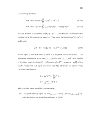
177. 147
• executing Laplacian average consensus until the agents’ estimates fall within
a centered interval around the average of the initial conditions; and
• running two agreement protocols on the minimum of quantities computed by
the agents.
5.4 Simulation example
Here we simulate1 the performance of the Consensus-based Saddle-Point
(Sub-) Gradient algorithm (cf. Algorithm 1) in a network of N = 50 agents whose
communication topology is given by a fixed connected small world graph [WS98]
with maximum degree dmax = 4. Under this coordination strategy, the 50 agents
solve collaboratively the following instance of problem (5.2) with nonlinear convex
constraints:
min
wi∈[0,1]
50
i=1
ciwi
s.t.
50
i=1
−di log(1+wi) ≤ −b. (5.40)
Problems with constraints of this form arise, for instance, in wireless networks
to ensure quality-of-service. For each i ∈ {1,...,50}, the constants ci, di are
taken randomly from a uniform distribution in [0,1], and b = 5. We compute the
solution to this problem, to use it as a benchmark, with the Optimization Toolbox
using the solver fmincon with an interior point algorithm. Since the graph is
connected, it follows that B = 1 in the definition of joint connectivity. Also, the
constant of nondegeneracy is δ = 0.25 and σmax(L) ≈ 1.34. With these values, we
1The Matlab code is available at https://github.com/DavidMateosNunez/
Consensus-based-Saddle-Point-Subgradient-Algorithm.git.

178. 148
derive from (5.18) the theoretically feasible consensus stepsize σ = 0.2475. For the
projection step in (5.29d) of the C-SP-SG algorithm, the bound on the optimal
dual set (5.36), using the Slater vector ˜w = 1N and ¯z = 0, is
r =
N maxj∈{1,...,N} cj
log(2) N
i=1 di −N/10
= 3.313.
For comparison, we have also simulated the Consensus-Based Dual Decomposition
(CoBa-DD) algorithm proposed in [SJR16] using (and adapting to this problem)
the code made available online by the authors2. (The bound for the optimal dual
set used in the projection of the estimates of the multipliers is the same as above.)
We should note that the analysis in [SJR16] only considers constant learning rates,
which necessarily results in steady-state error in the algorithm convergence.
We have simulated the C-SP-SG and the CoBa-DD algorithms in two
scenarios: under the Doubling Trick scheme of Assumption 2.31 (solid blue and
magenta dash-dot lines, respectively), and under constant learning rates equal
to 0.05 (darker grey) and 0.2 (lighter grey). Fig. 5.2 shows the saddle-point
evaluation error for both algorithms. The saddle-point evaluation error of our
algorithm is well within the theoretical bound established in Corollary 3.34, which
for this optimization problem is approx. 1.18×109/
√
t. (This theoretical bound
is overly conservative for connected digraphs because the ultimate bound for
the disagreement Cu in (5.20), here Cu ≈ 3.6 × 106, is tailored for sequences of
digraphs that are B-jointly connected instead of relying on the second smallest
eigenvalue of the Laplacian of connected graphs.) Fig. 5.3 compares the network
cost-error and the constraint satisfaction. We can observe that the C-SP-SG and
the CoBa-DD [SJR16] algorithms have some characteristics in common:
2The Matlab code is available at http://ens.ewi.tudelft.nl/~asimonetto/
NumericalExample.zip.

179. 149
• They both benefit from using the Doubling Trick scheme.
• They approximate the solution, in all metrics of Fig. 5.2 and Fig. 5.3 at
a similar rate. Although the factor in logarithmic scale of the C-SP-SG
algorithm is larger, we note that this algorithm does not require the agents
to solve a local optimization problem at each iteration for the updates of
the primal variables, while both algorithms share the same communication
complexity.
• The empirical convergence rate for the saddle-point evaluation error under
the Doubling Trick scheme is of order 1/
√
t (logarithmic slope −1/2), while
the empirical convergence rate for the cost error under constant learning rates
is of order 1/t (logarithmic slope −1). This is consistent with the theoretical
results here and in [SJR16] (wherein the theoretical bound concerns the
practical convergence of the cost error using constant learning rates).
5.5 Discussion
We have proposed provably correct projected subgradient methods for
saddle-point problems under explicit agreement constraints. We have shown that
separable constrained optimization problems can be written in this form, where
agreement plays a role in making the objectives (via agreement on a subset of the
primal variables) as well as the constraints (via agreement on the dual variables)
distributed. This approach enables the use of existing consensus-based ideas to
tackle the algorithmic solution to these problems in a distributed fashion. We
have illustrated how the general saddle-point formulation adopted in this paper
encompasses optimization problems with separable and semidefinite constraints.

180. 150
Iteration, t
100
102
104
106
10−3
10−2
10−1
100
101
CoBa-SPS
CoBa-DD
Figure 5.2: Saddle-point evaluation error |φφφ(wwwav
t ,zzzav
t )−L(www∗,z∗)|. The lines
in grey represent the same algorithms simulated with constant learning rates
equal to 0.2 (lighter grey) and 0.05 (darker grey), respectively.
Acknowledgments
This chapter is taken from a work submitted by D. Mateos-Núñez and
J. Cortés to IEEE Transactions on Automatic Control, with the title “Distributed
saddle-point subgradient algorithms with Laplacian averaging.” A preliminary
version will appear in the Proceedings of the IEEE Conference on Decision and
Control, Osaka, Japan, to be held in December 2015. This research was supported
by the US National Science Foundation (NSF) Award CMMI-1300272.

181. 151
Iteration, t
100
102
104
106
10−7
10−6
10−5
10−4
10−3
10−2
10−1
100
101
CoBa-SPS
CoBa-DD
(a) Cost error
Iteration, t
100
102
104
106
10−7
10−6
10−5
10−4
10−3
10−2
10−1
100
101
CoBa-SPS
CoBa-DD
(b) Constraint satisfaction
Figure 5.3: Cost error and constraint satisfaction. For the same instan-
tiations as in Fig. 5.2, (a) represents the evolution of the network cost er-
ror | N
i=1 ci(wi
t)
av
− N
i=1 ciw∗
i |, and (b) the evolution of the network constraint
satisfaction − N
i=1 di log(1+(wi
t)
av
)+b.

182. Chapter 6
Distributed optimization for
multi-task learning via
nuclear-norm approximation
In this chapter we finish our incursions in distributed optimization. Here we
exploiting a variational characterization of the nuclear norm to extend the framework
of distributed convex optimization to machine learning problems that focus on
the sparsity of the aggregate solution. We propose two distributed dynamics
that can be used for multi-task feature learning and recommender systems in
scenarios with more tasks or users than features. Our first dynamics tackles a
convex minimization on local decision variables subject to agreement on a set of
local auxiliary matrices. Our second dynamics employs a saddle-point reformulation
through Fenchel conjugation of quadratic forms, avoiding the computation of the
inverse of the local matrices. We establish the correctness of both coordination
algorithms using the general analytical framework of the previous chapter. Finally,
we illustrate these results in a simulation example of low-rank matrix completion.
152

183. 153
6.1 Optimization with nuclear norm regulariza-
tion
We are interested in developing distributed coordination algorithms to solve
the optimization problem
min
wi∈W,
i∈{1,...,N}
N
i=1
fi(wi)+γΩ(W), (6.1)
where W ⊆ Rd is a closed convex set; the matrix W ∈ Rd×N aggregates the vectors
{wi}N
i=1 as columns, i.e., W := [w1|...|wN ]; each function fi : Rd → R is convex;
γ ∈ R>0 is a design parameter; and Ω : Rd×N → is a joint regularizer to promote
solutions with low rank or other sparsity patterns. We next motivate the distributed
optimization problem with nuclear-norm regularization in two scenarios.
6.1.1 Multi-task feature learning
In data-driven optimization problems each function fi often codifies the
loss incurred by the vector of weighting parameters wi with respect to a set of
ni data points {pj,yj}ni
j=1. As such, this loss can be called residual or margin,
depending on whether we are considering regression or classification problems. The
work [AEP08] exploits the relation (2.10) as follows. For a given W ∈ Rd×N , the
following regularizer is used,
Ω(W) = min
U∈Od
,A∈Rd×N
W=UA
A 2,1
= min
U∈Od
W U 2,1 = W ∗.

184. 154
This minimization promotes a dictionary matrix U of orthonormal columns such
that the columns of W are sparse linear combinations of them. The latter is
achieved through A 2,1, which ‘favors’ rows of small size because the one-norm
is the convex surrogate of the zero-norm, or number of nonzero elements. This
offers an interesting perspective on minimization problems that are convex on
the product UA, with U ∈ Od, and have a penalty term A 2,1. As pointed
in [AEP08], the above characterization enables a convex reformulation on the
matrix variable W = UA.
6.1.2 Matrix completion for recommender systems
The estimation of a low-rank matrix from a set of entries, or matrix com-
pletion, see, e.g., [MHT10], also fits naturally in the framework of (6.1) with
nuclear-norm regularization. This is because the nuclear norm is the convex surro-
gate of the rank function [Faz02]. Let Z ∈ Rd×N be a low-rank matrix of unknown
rank for which only a few entries per column are known. The goal is then to
determine a matrix W that minimizes the Frobenius norm across the revealed
entries while keeping small the nuclear norm,
min
wi∈W,
i∈{1,...,N}
N
i=1j∈Υi
(Wji −Zji)2
+γ W ∗ (6.2)
where, for each i ∈ {1,...,N},
Υi := {j ∈ {1,...,d} : Zji is a revealed entry of Z}.

185. 155
6.1.3 A case for distributed optimization
The optimization problem (6.1) can be formulated as a convex and separable
minimization when the joint regularizer is · ∗ or · 2
∗ using the characteriza-
tions (2.8a) or (2.8b). Assuming that a minimum exists, we can write
min
W∈Rd×N
N
i=1
fi(wi)+γ W 2
∗
= min
W∈Rd×N
D∈Sd
0, trace(D)≤1
wi∈C(D),∀i
N
i=1
fi(wi)+γ
N
i=1
wi D†
wi .
= min
wi∈W,∀i
Di∈Sd
0, trace(Di)≤1, ∀i
wi∈C(Di), ∀i
Di=Dj, ∀i,j
N
i=1
fi(wi)+γ
N
i=1
wi D†
i wi , (6.3)
and similarly for Ω(W) = 2 W ∗ replacing the constraint trace(D) ≤ 1 by the
penalty functions γ N
i=1
1
N trace(Di). When d N, it is reasonable to design
distributed strategies that use local gradient descent and consensus to solve this
problem because the objective can be split across a network of agents, and the only
coupling constraint is the agreement on the matrix arguments, Di = Dj for each
i, j, whose dimensions do not grow with the network size. The condition d N
in multi-task feature learning implies that there are far less features than tasks or
users (for instance, there are less diseases or symptoms than people). The same
observation applies to matrix completion in collaborative filtering where the rows
represent features and the columns represent users.
However, the design of distributed strategies to solve (6.3) raises the following
challenges,
(i) The constraint set {w ∈ Rd,D ∈ Sd
0 : w ∈ C(D)} is convex but not closed,
which is a difficulty when designing a projection among the local variables.

186. 156
Note that for any fixed matrix Di, one could project wi onto C(Di) by
computing DiD†
i w, but this projection is state-dependent.
(ii) The computation of D†
i is a concern because Di might be rank deficient and
the pseudoinverse might be discontinuous when the rank of Di changes.
We avoid these difficulties by enforcing the solution to be within a margin of
the boundary of the positive semidefinite cone. This is achieved by considering an
approximate regularization that we introduce in Section 6.2.1. Our first dynamics
solves the nuclear-norm regularization as a separable minimization with agreement
constraint. Even with (ii) addressed, an additional challenge involves the efficient
computation of the inverse:
• Iterative algorithms involving the computation of D−1 are computationally
expensive and potentially lead to numerical instabilities.
We eliminate the necessity of computing D−1 altogether in Section 6.2.2 by trans-
forming the convex minimization into a saddle-point problem. This transformation
is general and does not require the approximate treatment of the nuclear norm
regularization in Section 6.2.1. Our second dynamics solves the nuclear-norm
regularization as a separable min-max problem with agreement constraint.
6.2 Distributed coordination algorithms
Here we address the three challenges outlined in Section 6.1 to solve the
optimization problem (6.3). In the forthcoming discussion, we present two refor-
mulations of this problem and two distributed coordination algorithms to solve
them.

187. 157
6.2.1 Nuclear norm approximate regularization
In relation to the first two challenges outlined above, note that the optimal
values D∗
1 and D∗
2 in (2.9) for the variational characterizations of · ∗ and · 2
∗
are in general positive semidefinite. To enforce these optimal values to be in
the interior of the positive semidefinite cone, following the technique in [AEP08,
Sec. 4], we consider an approximate problem by introducing in (6.3) the barrier
function trace(D†) for some ∈ R>0. We next justify how the optimizer of the
approximate problem, which depends on , is farther than some margin from the
boundary of Sd
0 (in turn, this fact allows to insert in our optimization problem a
dummy constraint of the form D cI, where c is what we refer to as the margin).
For Ω (W) = 2 [W|
√
Id] ∗, this is easy to see because, in view of (2.9),
D∗
1, := WW + Id
√
Id.
For Ω (W) = [W|
√
Id] 2
∗, we need more care and we offer next a result using the
notation for the reduced spectraplex defined in Section 2.4.
Lemma 2.37. (Dummy constraint for -approximate regularization under Ω(W) =
W 2
∗). Let W ∈ Rd×N be any matrix whose columns have two-norm bounded by rw.
Then, the optimizer of
min
D∈Sd
0,trace(D)≤1,
C(W)⊆C(D)
trace D†
(WW + I) , (6.4)
(whose optimal value is [W |
√
Id ] 2
∗), also minimizes
min
D∈∆(c )
trace D†
(WW + I) ,

188. 158
where the margin c of the reduced spectraplex ∆(c ) is
c :=
√
√
d Nr2
w + d
. (6.5)
Furthermore, c in (6.5) satisfies c ≤ 1/d for any ,rw ∈ R>0. Hence, ∆(c ) is
nonempty for any ,rw ∈ R>0.
Proof. In view of (2.8b) and (2.9), the optimizer of (6.4) is
D∗
2, :=
√
WW + Id
trace( WW + Id)
. (6.6)
Using the inequality for the nuclear and the Frobenius norm (2.3), we have
D∗
2, =
√
WW + Id
[W |
√
Id ] ∗
≥
√
√
d [W |
√
Id ] F
Id
=
√
√
d W 2
F +
√
Id
2
F
Id ≥
√
√
d Nr2
w + d
Id ,
where in the last two equations we have used the fact that the square Frobenius norm
is the sum of square two-norms of the columns. The second fact is trivial.
As a result, when we add the barrier terms N
i=1 N trace(D†
i ) to the optimiza-
tion in (6.3), the constraints Di ∈ Sd
0 and wi ∈ C(Di) can be replaced by Di c Id.
Hence, the variational characterization of [W |
√
Id ] 2
∗ can be written over the
compact domain ∆(c ). Alternatively, in the case of 2 [W |
√
Id ] ∗, we saw above
that we can use the constraint Di
√
Id to achieve the same effect. However,
because the trace constraint is now absent, we construct a compact domain contain-
ing the optimal value D∗
1, by introducing one more dummy constraint Di F ≤ r ,

189. 159
with
r :=
√
Nrw +
√
d. (6.7)
This, together with the constraint Di
√
Id, yields the compact domain given
by the reduced ice-cream D(
√
,r ). The derivation is similar to the proof of
Lemma 2.37; here we compute an upper bound as opposed to a lower bound. In both
cases, we use the fact that the columns of W are contained in the ball ¯B(0,rw) ⊆ Rd.
The following results summarizes our discussion above.
Corollary 2.38. (Separable minimization with agreement constraint). Let W ∈
¯B(0,rw) and define c as in (6.5). Then
min
W∈Rd×N
N
i=1
fi(wi)+γΩ (W), (6.8)
with Ω (W) = [W |
√
Id ] 2
∗ is equal to
min
wi∈W,∀i,
Di∈∆(c ), ∀i,
Di=Dj, ∀i,j
N
i=1
fi(wi)+γ
N
i=1
wi D−1
i wi + N trace(D−1
i ) . (6.9)
The analogous result is valid for Ω (W) = 2 [W |
√
Id ] ∗ replacing ∆(c ) by D(
√
,r )
and including the penalty functions γ N
i=1
1
N trace(Di).
In both cases of Corollary 2.38, Weierstrass’ Theorem guarantees that the
minimum is reached since we are minimizing a continuous function over a compact
set. This leads to our first candidate dynamics.

190. 160
Distributed subgradient dynamics for nuclear optimization.
Our first coordination algorithm for the distributed optimization with nu-
clear norm (6.8) is a subgradient algorithm with proportional feedback on the
disagreement on the matrix variables:
ˆwi(k +1) =wi(k)−ηk gi(k)+2γDi(k)−1
wi(k) ,
ˆDi(k +1) =Di(k)−ηkγ −D−1
i (k)wi(k)wi(k) D−1
i (k)
+ α
N Id − N D−2
i (k) +σ
N
j=1
aij,t(Dj(k)−Di(k)),
wi(k +1) =PW( ˆwi(k +1)),
Di(k +1) =PD( ˆDi(k +1)), (6.10)
where gi(k) ∈ ∂fi(wi(k)), for each i ∈ {1,...,N}, and PW(·) and PD(·) denote the
projections onto the compact convex sets W and D. This notation allows us to
consider both approximate regularizers: for the case 2 [W |
√
Id ] ∗, the trace acts
as a penalty, i.e., α = 1, and the domain is D = D(
√
,r ); for the case [W |
√
Id ] 2
∗,
the trace acts as a constraint, i.e., α = 0, and D = ∆(c ).
Remark 2.39. (Implementation of the orthogonal projections). The fact that
projections need to be orthogonal raises additional conceptual challenges. We make
here the following observations:
• If we represent the set D(c,r) as the intersection {D ∈ Sd : D cId}∩{D ∈
Rd×d : D F ≤ r}, then a candidate projection onto D(
√
,r ) can be per-
formed by the composition of a matrix square root,
P{D∈Sd :D cId}(D) = (D −cId)2 +cId,

191. 161
and, if D F ≥ r , the normalization step
P ¯BF (0,r )(D) :=
r
D F
D.
(The matrix square root can be computed efficiently using Newton method [Hig86].)
Each of these functions is an orthogonal projection onto the corresponding
set. However, each of them is guaranteed to preserve the set of the other only
if c = 0. This implies that, in general, they need to be applied iteratively.
• Similar considerations apply to the projection onto ∆(c), but in contrast
with D(c,r), the orthogonal projections onto {D ∈ Sd : D cId}, and {D ∈
Rd×d : trace(D) ≤ 1} do not preserve each other’s corresponding sets even
when c = 0. •
6.2.2 Separable saddle-point formulation
In the previous section we have written the optimization (6.8) with approx-
imate nuclear norm regularization as a separable convex optimization with an
agreement constraint on auxiliary local matrices. Here we derive an equivalent
min-max problem that is also separable and has the advantage of enabling iterative
distributed strategies that avoid the computation of the inverse of the local ma-
trices. To achieve this aim, the next result expresses the quadratic forms w D†w
and trace(D†) = d
j=1 ej D†ej as the maximum of concave functions in additional
auxiliary variables. We write these expressions using Fenchel conjugacy of quadratic
forms, and in doing this, we avoid the need to compute the pseudoinverse of D.
Proposition 2.40. (Min-max formulation via Fenchel conjugacy). For i ∈ {1,...,N}

192. 162
and α ∈ R≥0, let Fi : W ×Rd×d ×Rd ×Rd×d → R be defined by
Fi (w,D,x,Y ) := fi(w)+γ trace D(−xx − N Y Y )
−2γw x−2γ
N
trace(Y )+
α
N
trace(D). (6.11)
Then, the following two optimizations are equivalent
min
D∈Sd
0,
w∈W∩C(D)
fi(w)+γ w D†
w + N trace(D†
)+ α
N trace(D)
= min
w∈W,D∈Rd×d
sup
x∈Rd,Y ∈Rd×d
Fi(w,D,x,Y ). (6.12)
Moreover, the minimization on the right does not change with the addition of
the constraints D ∈ Sd
0 and w ∈ C(D) (which allows to replace the operator sup
by max).
Proof. For any w ∈ W and D ∈ Rd×d, it holds that
sup
x∈Rd
−(x Dx+2w x) =



w D†w if D ∈ Sd
0 ,w ∈ C(D),
∞ otherwise.
This transformation is the same as Fenchel conjugacy up to a factor, see, e.g., [BV09,
P. 649]. When D ∈ Sd
0 and w ∈ C(D), the maximizer is x∗ = −D†w. Since
w D†
w +
N
trace(D†
) = w D†
w +
N
d
j=1
ej D†
ej ,

193. 163
this term can be substituted in the minimization (6.12) by
sup
x∈Rd
−(x Dx+2w x)+
N
d
j=1
sup
yj∈Rd
−(yj
Dyj
+2ejyj
)
= sup
x∈Rd,Y ∈Rd×d
−x Dx−2w x
−
N
trace(DY Y )−
2
N
trace(Y ) ,
where Y = [y1|···|yd ] ∈ Rd×d, completing the proof.
The function w D†w is jointly convex in the convex domain {w ∈ W, D ∈
Sd
0 : w ∈ C(D)} because it is a point-wise maximum of linear functions indexed by
x. (The function is also proper but not closed because the domain is not closed).
The same considerations apply adding the constraint trace(D) ≤ 1. We are now
ready to establish the main equivalence between optimization problems.
Corollary 2.41. (Separable min-max problem with agreement constraint).. The
optimization (6.8) with Ω (W) = [W |
√
Id ] 2
∗ is equivalent to
min
wi∈W,Di∈Rd×d
,
trace(Di)≤1, ∀i,
Di=Dj ∀i,j
sup
xi∈Rd
,∀i
Yi∈Rd×d
,∀i
N
i=1
Fi(wi,Di,xi,Yi), (6.13)
without the penalty on the trace in Fi (i.e., α = 0) for each i ∈ {1,...,N}. As long as
c is given by (6.5) and W ⊆ ¯B(0,rw), the constraints Di ∈ ∆(c ) are not necessary,
but including them allows to replace the operator sup by max. An analogous result
holds for Ω (W) = 2 [W |
√
Id ] ∗ when, instead of the trace constraints, one has
the penalty terms N
i=1
1
N trace(Di) (i.e., α = 1). In this case, as long as r is given
by (6.7) and W ⊆ ¯B(0,rw), the constraints Di ∈ D(
√
,r ) are not necessary.
Proof. The proof for both cases is analogous so, for brevity, we only present it

194. 164
for Ω (W) = [W |
√
Id ] 2
∗. Introducing the constraint trace(D) ≤ 1 on both sides
of (6.12), and adding over i = 1,...,N under the agreement constraint Di = Dj for
each 1 ≤ i, j ≤ N, we get
min
wi∈W,∀i,
Di∈Sd
0, trace(Di)≤1, ∀i,
wi∈C(Di), ∀i,
Di=Dj, ∀i,j
N
i=1
fi(wi)
+γ
N
i=1
wi D†
i wi + N trace(D†
i )
= min
wi∈W, ∀i,
Di∈Rd×d
, trace(Di)≤1, ∀i,
Di=Dj ∀i,j
max
xi∈Rd
,∀i
Yi∈Rd×d
,∀i
N
i=1
Fi(wi,Di,xi,Yi).
On the right hand side the solution does not change if we introduce the constraints
Di ∈ Sd
0, wi ∈ C(Di) thanks to Proposition 2.40. Moreover, the solution remains
also the same by substituting both constraints on either side by D ∈ ∆(c ) thanks
to Lemma 2.37 as long as c is given by (6.5) and W ∈ ¯B(0,rw).
The next result establishes the existence of a saddle-point for the convex-
concave formulation of the -approximate minimization. For convenience, de-
fine F : WN ×∆(c )×(Rd)N ×(Rd×d)N → R as
F(www,D,xxx,YYY ) :=
N
i=1
Fi(wi,D,xi,Yi), (6.14)
where www := (w1,...wN ), xxx := (x1,...xN ), YYY := (Y1,...YN ).
Proposition 2.42. (Existence of saddle points). For W ⊆ ¯B(0,rw) and D equal
to either ∆(c ) or D(
√
,r ), the set of saddle points of F on WN ×D ×(Rd)N ×

195. 165
(Rd×d)N is nonempty and compact, and, as a consequence,
max
xi∈Rd,Yi∈Rd×d,∀i
min
wi∈W,∀i,D∈∆(c )
N
i=1
Fi(wi,D,xi,Yi)
= min
wi∈W,∀i,D∈∆(c )
max
xi∈Rd,Yi∈Rd×d,∀i
N
i=1
Fi(wi,D,xi,Yi).
(The agreement constraints Di = Dj for all i,j ∈ {1,...,N} are written implic-
itly because the existence of saddle-points is established within those agreement
constraints.)
Proof. We use the Saddle-Point Theorem [BNO03, Thm. 2.6.9, p. 150]. First
we need to verify the hypotheses of [BNO03, Assumption 2.6.1, p. 144]. For
each (xxx,Y ) ∈ (Rd)N ×(Rd×d)N , we introduce the function txxx,YYY : WN ×D → R∪{∞}
defined by
txxx,YYY (www,D) :=



F(www,D,xxx,YYY ) if (www,D) ∈ WN ×D,
∞ if (www,D) /∈ WN ×D,
and for each (www,D) ∈ WN ×D, we introduce the function rwww,D : (Rd)N ×(Rd×d)N →
R∪∞ given by
rwww,D(xxx,YYY ) := −F(www,D,xxx,YYY ).
We observe that for each (xxx,YYY ) ∈ (Rd)N ×(Rd×d)N , the function txxx,YYY is closed and
convex, and similarly, for each (www,D) ∈ WN ×D, the function rwww,D is also closed
and convex. Hence the aforementioned assumption holds. Going back to [BNO03,
Thm. 2.6.9, p. 150], we verify that the set WN ×D is compact, and the last step is

196. 166
to show that there exists (¯www, ¯D) ∈ WN ×D and α ∈ R such that the level set
{(xxx,YYY ) ∈ (Rd
)N
×(Rd×d
)N
: F(¯www, ¯D,xxx,YYY ) ≥ α} (6.15)
is nonempty and compact. We first prove that is closed, then that is bounded,
and finally that is nonempty for some α ∈ R. The level set is closed because
F is continuous. To show that is bounded, we will prove that it is contained
in a ball. For this, we use [Ber05, Prop 8.4.13] on the trace of a product of a
symmetric matrix and a positive semidefinite matrix, which can be bounded as
trace( ¯DY Y ) ≤ λmax( ¯D)trace(Y Y ) ≤ trace(Y Y ) = Y 2
F because trace( ¯D) ≤ 1
and ¯D 0, and similarly we bound x ¯Dx ≤ x 2
2. Therefore,
F(¯www, ¯D,xxx,YYY )−
N
i=1
fi( ¯wi)
=γ
N
i=1
trace ¯D(−xixi − N YiYi + α
N )
−2 ¯wi xi −2N trace(Yi)
≥ −γ
N
i=1
xi
2
2 + N Yi
2
F + αd
N +2 ¯wi xi +2N trace(Yi)
≥ −γ
N
i=1
2 xi
2
2 +r2
w +2N Yi
2
F +(α+ ) d
N ,
where in the last inequality we have used that 2trace(Y ) ≤ d+trace(Y Y ), which
follows because
0 ≤ Id −Y 2
F = trace(I−Y )(I−Y )
= trace(Id +Y Y −Y −Y ) = d+ Y 2
F −2trace(Y ),
and, similarly, 2 ¯wi x ≤ ¯wi
2
2 + x 2
2 ≤ r2
w + x 2
2. Therefore, the level set in (6.15)

197. 167
is contained in the set
(xxx,YYY ) ∈ (Rd
)N
×(Rd×d
)N
:
c∗
−γ
N
i=1
2 xi
2
2 +r2
w +2N Yi
2
F + N d ≥ α , (6.16)
where c∗ := minwww∈WN
N
i=1 fi(wi). Note that c∗ is well defined thanks to Weierstrass’
Theorem. The boundedness of the set (6.15) then follows because the super set (6.16)
is bounded for any α ∈ R (although it may be empty). Finally, we need to find some
α for which the level set in (6.15) is nonempty. For this, note that the point (xxx,YYY ) =
(0Nd,0d×Nd) belongs to the level set (6.15) for α ≤ N
i=1 fi( ¯wi) = F(¯www, ¯D,0,0). (We
could have shown that in fact for any (¯xxx, ¯YYY ) ∈ (Rd)N ×(Rd×d)N there exists ¯α such
that (¯xxx, ¯YYY ) is in the level set of level ¯α, but this is not required.)
The above discussion leads us to introduce our second candidate dynamics.
Distributed saddle-point dynamics for nuclear optimization.
Our second coordination algorithm for the distributed optimization with nu-
clear norm (6.8) is a saddle-point subgradient dynamics with proportional feedback
on the disagreement of a subset of the variables:
wi(k +1) =PW wi(k)−ηk gi(k)−2γxi(k) ,
Di(k +1) =PD Di(k)−ηkγ −xixi − N YiYi + α
N Id
+σ
N
j=1
aij,t(Dj(k)−Di(k)) ,
xi(k +1) =xi(k)+ηkγ −2Dixi(k)−2wi(k) ,
Yi(k +1) =Yi(k)+ηkγ −
2
N
Di(k)Yi(k)−
2
N
Id , (6.17)

198. 168
where gi(k) ∈ ∂fi(wi(k)), for each i ∈ {1,...,N}, and PW(·) and PD(·) denote
the projections onto the compact convex sets W and D. For the case of the
regularizer 2 [W |
√
Id ] ∗ we set α = 1 and D = D(
√
,r ), and for the regularizer
[W |
√
Id ] 2
∗, we set α = 0 and D = ∆(c ).
6.3 Convergence analysis
The convergence result of the distributed strategies (6.10) and (6.17) follows
from Theorem 2.32, as we outline next.
Theorem 3.43. (Convergence of the coordination algorithms (6.10) and (6.17)).
Let the convex compact set W ⊆ Rd be contained in ¯B(0,rw) and let the bounds c
and r be defined as in (6.5) and (6.7). Assume that each dynamics evolves over a
sequence {Gt}t≥1 of B-jointly connected, δ-nondegenerate, weight-balanced digraphs
with uniformly bounded Laplacian eigenvalues. Let σ be as follows: for any ˜δ ∈ (0,1),
let ˜δ := min ˜δ , (1− ˜δ ) δ
dmax
, where dmax := max dout,t(j) : j ∈ I, t ∈ Z≥1 , and
choose
σ ∈
˜δ
δ
,
1− ˜δ
dmax
.
Assume also that the learning rates be chosen according to the Doubling Trick
in Assumption 2.31. Then both the dynamics (6.10) and (6.17) converge to an
optimizer of (6.8). The evaluation error with respect to any minimum of (6.9), or
with respect to any saddle point of the convex-concave function (6.13), is proportional
to 1/
√
t.
Proof. The convergence result for both dynamics follows from the results in The-
orem 2.32. Regarding the dynamics (6.17), the hypotheses of Theorem 2.32 are

199. 169
satisfied as we summarize next: the existence of a saddle point is proved in Propo-
sition 2.42; the evolution of the estimates {wi(k)}N
i=1 and {Di(k)}N
i=1 in (6.17) is
uniformly bounded thanks to the projections onto the compact sets W and ∆(c ).
On the other hand, the auxiliary states {xi(k)}N
i=1 and {Yi(k)}N
i=1 are uniformly
bounded by virtue of Proposition 3.44 below. As a consequence of the bounded
evolution of the dynamics (6.17), one can also construct bounds for the subgra-
dients of each convex-concave function Fi. The other assumptions regarding the
communication graphs and the choice of the design parameters σ and the learning
rates {ηt}t≥1 complete the hypotheses in Theorem 2.32. The convergence follows
similarly from this result for the dynamics (6.10), which is also a particular case of
the general dynamics (5.6).
The proof of correctness above requires the evolution of the estimates of
the dynamics to be bounded. In particular, the current analysis establishes the
boundedness of the auxiliary states {xi(k)}N
i=1 and {Yi(k)}N
i=1 in the dynamics (6.17)
by heavily relying on the fact that wi(k) ∈ ¯B(0,rw) and Di(k) cId for all k ≥ 1.
Precisely, we use the latter to show the input-to-state stability (ISS) property
(see [JSW99]) of the system
xk+1 =xk +ηkγ −2Dkxk −2wk , (6.18a)
Yk+1 =Yk +ηkγ −
2
N
DkYk −
2
N
Fk , (6.18b)
for arbitrary sequences of disturbances {wk}k≥1 ⊂ Rd and {Fk}k≥1 ⊂ Rd×d, where
Dk cId.
Proposition 3.44. (ISS Lyapunov function for the auxiliary states in (6.17)).
Assume Dk cId and Dk 2 ≤ r for some c ∈ R>0 and r ∈ [1,∞), respectively, and

200. 170
let {ηk} ⊂ R>0 be any sequence of learning rates such that
ηk ≤ min
c−κ
4γr2
,
N(c−κ)
4γ r2
, (6.19)
for some κ ∈ (0,c) for all k ≥ 1. Then, the function · 2
2 is an ISS-Lyapunov
function for the evolution of xk in (6.18a) when {wk}k≥1 ⊂ Rd is considered as a
sequence of disturbances,
xk+1
2
2 ≤ 1−ηkγκ xk
2
2 + 8η2
kγ2
+
ηkγ
κ
wk
2
2 ,
for all k ≥ 1. Similarly, the function · 2
F is an ISS Lyapunov function for the
evolution of Yk in (6.18b) under the sequence of disturbances {Fk}k≥1 ⊂ Rd×d,
Yk+1
2
F ≤ 1−
ηkγκ
N
Yk
2
F +
8η2
kγ2 2
N2
+
ηkγ
κN
Fk
2
F ,
for all k ≥ 1.
Proof. Taking the square norm on both sides of the dynamics (6.18a), we get
xk+1
2
2 = xk +ηkγ −2Dkxk −2wk
2
2
= xk
2
2 +4η2
kγ2
Dkxk +wk
2
2 −2ηkγxk (Dkxk +wk).
Next we use Young’s inequality, 2x w ≤ κ x 2
2 + 1
κ w 2
2, for any κ ∈ R>0 and all
x,w ∈ Rd,
xk+1
2
2 − xk
2
2 ≤η2
kγ2
Dkxk +wk
2
2 −2ηkγxk Dkxk
+ηkγκ xk
2
2 +
ηkγ
κ
wk
2
2
≤ −ηkγ 2c−κ−8ηkγr2
xk
2
2 + 8η2
kγ2
+
ηkγ
κ
wk
2
2 , (6.20)

201. 171
where in the last inequality we have used that Dk cId and also
Dkxk +wk
2
2 ≤2 Dkxk
2
2 +2 wk
2
2
≤2 Dk
2
2 xk
2
2 +2 wk
2
2 ≤ 2max{1,r2
} xk
2
2 +2 wk
2
2 ,
which follows by Young’s inequality. The first term in the minimum of (6.19) comes
then from imposing the condition 2c−κ−8ηkγr2 ≥ κ in (6.20).
We derive the analogous result for the dynamics (6.18a) using the Frobe-
nius norm · F in place of the Euclidean norm · 2 and using the inequality
trace(D W) ≤ κ D 2
F + 1
κ W 2
2. (This inequality is the same as for vectors be-
cause the Frobenius norm of a matrix is the Euclidean norm of the vectorization of
the matrix and the trace of the product of two matrices is the same as the scalar
product of the vectorization of the matrices.)
Yk+1
2
F = Yk
2
F +
4η2
kγ2 2
N2
DkYk +Fk
2
F
−
2ηkγ
N
trace Yk (DkYk +Fk)
so, using that −trace(Yk DkYk) ≤ −c Yk F ,
Yk+1
2
F − Yk
2
F ≤
4η2
kγ2 2
N2
DkYk +Fk
2
F
−
2ηkγ
N
trace Yk DkYk +
ηkγκ
N
Yk
2
F +
ηkγ
κN
Fk
2
F
≤ −
ηkγ
N
2c−κ−8
ηkγ r2
N
Yk
2
F +
8η2
kγ2 2
N2
+
ηkγ
κN
Fk
2
F ,
(6.21)

202. 172
where in the last inequality we have used again that Dk cId and also
DkYk +Fk
2
F ≤2 DkYk
2
F +2 Fk
2
F
≤2 Dk
2
F Yk
2
F +2 Fk
2
2 ≤ 2max{1,r2
} Yk
2
F +2 Fk
2
F ,
which follows by Young’s inequality as above. The second term in the minimum
of (6.19) comes from imposing 2c−κ−8ηkγ r2
N ≥ κ in (6.21).
As a consequence of the above result, the dynamics of xk and Yk in (6.18)
are ISS [JSW99, Lemma 3.5 and Remark 3.6]. The ISS property in turn implies
the uniform boundedness of the auxiliary states because in the dynamics (6.17),
we have wk ∈ ¯B(0,rw) and Fk = Id for all k ≥ 1.
6.4 Simulation example
Here we illustrate the performance of the distributed saddle-point algo-
rithm (6.17) on a matrix completion problem, cf. Section 6.1.2. The matrix
Z ∈ R8×20 has rank 2 and each agent is assigned a column. From each column,
only 5 entries have been revealed, and with this partial information, and with-
out knowledge about the rank of Z, the agents execute the coordination algo-
rithm (6.17) to solve the optimization (6.2). In this application each local function
fi(wi) = j∈Υi
(Wji − Zji)2 is not strongly convex, but just convex, in line with
the hypotheses of Theorem 3.43. Figure 6.1 illustrates the matrix fitting error, the
evolution of the network cost function, and the disagreement of the local auxiliary
matrices.

203. 173
6.5 Discussion
We have considered a class of optimization problems that involve the joint
minimization over a set of local variables of a sum of convex functions together
with a regularizing term that favors sparsity patterns in the resulting aggregate
solution. Particular instances of these optimization problems include multi-task
feature learning and matrix completion. We have exploited the separability prop-
erty of a variational characterization of the nuclear norm to design two types
of provably-correct distributed coordination algorithms. Our analysis relies on
the body of work on distributed convex optimization and saddle-point dynamics.
To the best of our knowledge, the proposed coordination algorithms are the first
distributed dynamics for convex optimization with nuclear-norm regularization.
Acknowledgments
This chapter is an extended version of a work by D. Mateos-Núñez and
J. Cortés presented in the IFAC Workshop on Distributed Estimation and Control
in Networked Systems, Philadelphia, Pennsylvania, USA, 2015, with the title
“Distributed optimization for multi-task learning via nuclear-norm approximation.”
The author of this thesis wishes to thank Ashish Cherukuri and Karan Sikka for
stimulating discussions during the creation of the manuscript, and Mariza Suárez for
her encouragement since the inception of these ideas. This research was supported
by NSF Award CMMI-1300272.

204. 174
10
0
10
1
10
2
10
3
10
4
0
0.5
1
1.5
2
Distributed saddle-point dynamics
Centralized subgradient descent
10
0
10
1
10
2
10
3
10
4
10
3
10
4
0 5000 10000 15000
0
1
2
3
4
5
iterations, k
W(k)−Z F
Z F
N
i=1 j∈Υi
(Wij(k)−Zij)2 +γ W(k)|
√
Id ∗
( N
i=1 Di(k)− 1
N
N
i=1 Di(k) 2
F )1/2
Figure 6.1: Simulation example of nuclear norm regularization for distributed
low-rank matrix completion. Here we represent the evolution of algorithm (6.17)
(magenta solid line). In the top we represent the matrix fitting error; in the center,
the evolution of network cost function, and, in the bottom, the disagreement of the
local matrices. The comparison is made with respect to a standard subgradient
descent algorithm (blue dashed line) with constant gradient stepsize equal to
0.1. (The subgradient of the nuclear norm employed therein takes the form
UrVr ∈ ∂ W(k) ∗, where UrΣrVr is the reduced singular value decomposition
of W(k).) The optimization parameter weighting the nuclear norm is γ = 2, and
the parameter of the approximate regularization is = 10−3. We use as constraint
set W = ¯B(0,rw) with rw = 800. In the distributed algorithm, the constraint set
for the auxiliary matrices is D = D(
√
,r ), the consensus stepsize is σ = 0.5, and
the communication topology is a ring connecting the 20 agents. Our algorithm
is slower because it halves the learning rates (subgradient stepsizes) according to
the doubling trick. This is necessary for asymptotic convergence in Theorem 3.43,
in sharp contrast with standard (centralized) gradient descent that uses constant
subgradient stepsize. The third plot shows the disagreement among the auxiliary
matrices for our distributed algorithm. For decreasing learning rates, which is
our case, the disagreement is guaranteed to converge to zero.

205. Chapter 7
pth moment noise-to-state
stability of stochastic differential
equations with persistent noise
We devote our last chapter to the stability properties of stochastic differential
equations subject to persistent noise (including the case of additive noise), which is
noise that is present even at the equilibria of the underlying differential equation
and does not decay with time. A condensed version of the main result of this
chapter was presented earlier in Section 2.6 because of its application to our
continuous-time distributed algorithm with noisy communication channels. The
class of systems we consider exhibit disturbance attenuation outside a closed,
not necessarily bounded, set. We identify conditions, based on the existence of
Lyapunov functions, to establish the noise-to-state stability in probability and in
pth moment of the system with respect to a closed set. As part of our analysis,
we study the concept of two functions being proper with respect to each other
formalized via pair of inequalities with comparison functions. We show that such
175

206. 176
inequalities define several equivalence relations for increasingly strong refinements
on the comparison functions. We also provide a complete characterization of the
properties that a pair of functions must satisfy to belong to the same equivalence
class. This characterization allows us to provide checkable conditions to determine
whether a function satisfies the requirements to be a strong NSS-Lyapunov function
in probability or a pth moment NSS-Lyapunov function.
7.1 Basic notions
We start with the basic definitions following [Mao11] with slightly more
detail than in Chapter 2.
7.1.1 Brownian motion
Throughout the chapter, we assume that (Ω,F,{Ft}t≥0,P) is a complete
probability space, where P is a probability measure defined on the σ-algebra F,
which contains all the subsets of Ω of probability 0. The filtration {Ft}t≥0 is a
family of sub-σ-algebras of F satisfying Ft ⊆ Fs ⊆ F for any 0 ≤ t < s < ∞; we
assume it is right continuous, i.e., Ft = ∩s>tFs for any t ≥ 0, and F0 contains all
the subsets of Ω of probability 0. The Borel σ-algebra in Rn, denoted by Bn, or
in [t0,∞), denoted by B([t0,∞)), are the smallest σ-algebras that contain all the
open sets in Rn or [t0,∞), respectively. A function X : Ω → Rn is F-measurable if
the set {ω ∈ Ω : X(ω) ∈ A} belongs to F for any A ∈ Bn. We call such function a
(F-measurable) Rn-valued random variable. If X is a real-valued random variable
that is integrable with respect to P, its expectation is E[X] = Ω X(ω)dP(ω). A
function f : Ω×[t0,∞) → Rn is F ×B-measurable (or just measurable) if the set
{(ω,t) ∈ Ω×[t0,∞) : f(ω,t) ∈ A} belongs to F ×B([t0,∞)) for any A ∈ Bn. We call

207. 177
such function an {Ft}-adapted process if f(.,t) : Ω → Rn is Ft-measurable for every
t ≥ t0. At times, we omit the dependence on “ω”, in the sense that we refer to the
indexed family of random variables, and refer to the random process f = {f(t)}t≥t0.
We define L1([t0,∞);Rn) as the set of all Rn-valued measurable {Ft}-adapted
processes f such that P({ω ∈ Ω : T
t0
f(ω,s) 2 ds < ∞}) = 1 for every T > t0.
Similarly, L2([t0,∞);Rn×m) denotes the set of all Rn×m-matrix-valued measurable
{Ft}-adapted processes G such that P({ω ∈ Ω : T
t0
G(ω,s) 2
F ds < ∞}) = 1 for
every T > t0.
A one-dimensional Brownian motion B : Ω × [t0,∞) → R defined in the
probability space (Ω,F,{Ft}t≥0,P) is an {Ft}-adapted process such that
• P({ω ∈ Ω : B(ω,t0) = 0}) = 1;
• the mapping B(ω,.) : [t0,∞) → R, called sample path, is continuous also with
probability 1;
• the increment B(.,t)−B(.,s) : Ω → R is independent of Fs for t0 ≤ s < t < ∞
(i.e., if Sb {ω ∈ Ω : B(ω,t)−B(ω,s) ∈ (−∞,b)}, for b ∈ R, then P(A∩Sb) =
P(A)P(Sb) for all A ∈ Fs and all b ∈ R). In addition, this increment is normally
distributed with zero mean and variance t−s.
An m-dimensional Brownian motion B : Ω × [t0,∞) → Rm is given by
B(ω,t) = [B1(ω,t),...,Bm(ω,t)] , where each Bi is a one-dimensional Brownian
motion and, for each t ≥ t0, the random variables B1(t),...,Bm(t) are independent.
7.1.2 Stochastic differential equations
Here we review some basic notions on stochastic differential equations (SDEs)
following [Mao11]; other useful references are [Kha12, Ö10, Mov11]. Consider the

208. 178
n-dimensional SDE
dx(ω,t) = f x(ω,t),t dt+G x(ω,t),t Σ(t)dB(ω,t), (7.1)
where x(ω,t) ∈ Rn is a realization at time t of the random variable x(.,t) : Ω → Rn,
for t ∈ [t0,∞). The initial condition is given by x(ω,t0) = x0 with probability 1
for some x0 ∈ Rn. The functions f : Rn ×[t0,∞) → Rn, G : Rn ×[t0,∞) → Rn×q,
and Σ : [t0,∞) → Rq×m are measurable. The functions f and G are regarded as a
model for the architecture of the system and, instead, Σ is part of the model for
the stochastic disturbance; at any given time Σ determines a linear transformation
of the m-dimensional Brownian motion {B(t)}t≥t0, so that at time t ≥ t0 the input
to the system is the process {Σ(t)B(t)}t≥t0, with covariance t
t0
Σ(t)Σ(t) ds. The
distinction between the roles of G and Σ is irrelevant for the SDE; both together
determine the effect of the Brownian motion. The integral form of (7.1) is given by
x(ω,t) = x0 +
t
t0
f x(ω,s),s ds+
t
t0
G x(ω,s),s Σ(s)dB(ω,s),
where the second integral is an stochastic integral [Mao11, p. 18]. A Rn-valued
random process {x(t)}t≥t0 is a solution of (7.1) with initial value x0 if
(i) is continuous with probability 1, {Ft}-adapted, and satisfies x(ω,t0) = x0
with probability 1,
(ii) the processes {f(x(t),t)}t≥t0 and {G(x(t),t)}t≥t0 belong to L1([t0,∞);Rn)
and L2([t0,∞);Rn×m) respectively, and
(iii) equation (7.1) holds for every t ≥ t0 with probability 1.
A solution {x(t)}t≥t0 of (7.1) is unique if any other solution {¯x(t)}t≥t0 with ¯x(t0) =
x0 differs from it only in a set of probability 0, that is, P( x(t) = ¯x(t) ∀t ≥ t0 ) = 1.

209. 179
We make the following assumptions on the objects defining (7.1) to guarantee
existence and uniqueness of solutions.
Assumption 1.45. We assume Σ is essentially locally bounded. Furthermore, for
any T > t0 and n ≥ 1, we assume there exists KT,n > 0 such that, for almost every
t ∈ [t0,T] and all x,y ∈ Rn with max x 2, y 2 ≤ n,
max f(x,t)−f(y,t) 2
2 , G(x,t)−G(y,t) 2
F ≤ KT,n x−y 2
2.
Finally, we assume that for any T > t0, there exists KT > 0 such that, for almost
every t ∈ [t0,T] and all x ∈ Rn, x f(x,t)+ 1
2 G(x,t) 2
F ≤ KT (1+ x 2
2).
According to [Mao11, Th. 3.6, p. 58], Assumption 1.45 is sufficient to
guarantee global existence and uniqueness of solutions of (7.1) for each initial
condition x0 ∈ Rn.
We conclude this section by presenting a useful operator in the stability
analysis of SDEs. Given a function V ∈ C2(Rn;R≥ 0), we define the generator of (7.1)
acting on the function V as the mapping L[V] : Rn ×[t0,∞) → R given by
L[V](x,t) V(x) f(x,t)+ 1
2 trace Σ(t) G(x,t) 2
V(x)G(x,t)Σ(t) . (7.2)
It can be shown that L[V](x,t) gives the expected rate of change of V along a
solution of (7.1) that passes through the point x at time t, so it is a generalization
of the Lie derivative. According to [Mao11, Th. 6.4, p. 36], if we evaluate V along
the solution {x(t)}t≥t0 of (7.1), then the process {V(x(t))}t≥t0 satisfies the new
SDE
V(x(t)) = V(x0)+
t
t0
L[V](x(s),s)ds+
t
t0
V(x(s)) G(x(s),s)Σ(s)dB(s). (7.3)

210. 180
Equation (7.3) is known as Itô’s formula and corresponds to the stochastic version
of the chain rule.
7.2 Noise-to-state stability via noise-dissipative
Lyapunov functions
In this section, we study the stability of stochastic differential equations
subject to persistent noise. Our first step is the introduction of a novel notion of
stability. This captures the behavior of the pth moment of the distance (of the
state) to a given closed set, as a function of two objects: the initial condition and
the maximum size of the covariance. After this, our next step is to derive several
Lyapunov-type stability results that help determine whether a stochastic differential
equation enjoys these stability properties. The following definition generalizes the
concept of noise-to-state stability given in [DK00].
Definition 2.46. (Noise-to-state stability with respect to a set). The system (7.1)
is noise-to-state stable (NSS) in probability with respect to the set U ⊆ Rn if for
any > 0 there exist µ ∈ KL and θ ∈ K (that might depend on ), such that
P |x(t)|p
U > µ |x0|U ,t−t0 +θ esssup
t0≤s≤t
Σ(s) F ≤ , (7.4)
for all t ≥ t0 and any x0 ∈ Rn. And the system (7.1) is pth moment noise-to-state
stable (pthNSS) with respect to U if there exist µ ∈ KL and θ ∈ K, such that
E |x(t)|p
U ≤ µ |x0|U ,t−t0 +θ esssup
t0≤s≤t
Σ(s) F , (7.5)
for all t ≥ t0 and any x0 ∈ Rn. The gain functions µ and θ are the overshoot gain

211. 181
and the noise gain, respectively.
The quantity Σ(t) F = trace Σ(t)Σ(t) is a measure of the size of the
noise because it is related to the infinitesimal covariance Σ(t)Σ(t) . The choice of
the pth power is irrelevant in the statement in probability since one could take any
K∞ function evaluated at |x(t)|U . However, this would make a difference in the
statement in expectation. (Also, we use the same power for convenience.) When
the set U is a subspace, we can substitute |.|U by . A, for some matrix A ∈ Rm×n
with N(A) = U. In such a case, the definition above does not depend on the choice
of the matrix A.
Remark 2.47. (NSS is not a particular case of ISS). The concept of NSS is not a
particular case of input-to-state stability (ISS) [Son08] for systems that are affine
in the input, namely,
˙y = f(y,t)+G(y,t)u(t) ⇔ y(t) = y(t0)+
t
t0
f(y(s),s)ds+
t
t0
G(y(s),s)u(s)ds,
where u : [t0,∞) → Rq is measurable and essentially locally bounded [Son98, Sec.
C.2]. The reason is the following: the components of the vector-valued function
t
t0
G(y(s),s)u(s)ds are differentiable almost everywhere by the Lebesgue fundamen-
tal theorem of calculus [MW99, p. 289], and thus absolutely continuous [MW99,
p. 292] and with bounded variation [MW99, Prop. 8.5]. On the other hand, at
any time previous to tk(t) min{t,inf {s ≥ t0 : x(s) 2 ≥ k}}, the driving distur-
bance of (7.1) is the vector-valued function
tk(t)
t0
G(x(s),s)Σ(s)dB(s), whose ith
component has quadratic variation [Mao11, Th. 5.14, p. 25] equal to
tk(t)
t0
m
j=1
|
q
l=1
G(x(s),s)ilΣ(s)lj|2
ds > 0.

212. 182
Since a continuous process that has positive quadratic variation must have infinite
variation [Kle05, Th. 1.10], we conclude that the driving disturbance in this case is
not allowed in the ISS framework. •
Our first goal now is to provide tools to establish whether a stochastic differ-
ential equation enjoys the noise-to-state stability properties given in Definition 2.46.
To achieve this, we look at the dissipativity properties of a special kind of energy
functions along the solutions of (7.1).
Definition 2.48. (Noise-dissipative Lyapunov function). A function V ∈ C2(Rn;R≥ 0)
is a noise-dissipative Lyapunov function for (7.1) if there exist W ∈ C(Rn;R≥ 0),
σ ∈ K, and concave η ∈ K∞ such that
V(x) ≤ η(W(x)), (7.6)
for all x ∈ Rn, and the following dissipation inequality holds:
L[V](x,t) ≤ −W(x)+σ Σ(t) F , (7.7)
for all (x,t) ∈ Rn ×[t0,∞).
Remark 2.49. (Itô formula and exponential dissipativity). Interestingly, the
conditions (7.6) and (7.7) are equivalent to
L[V](x,t) ≤ −η−1
(V(x))+σ Σ(t) F , (7.8)
for all x ∈ Rn, where η−1 ∈ K∞ is convex. Note that, since L[V] is not the Lie
derivative of V (as it contains the Hessian of V), one cannot directly deduce

213. 183
from (7.8) the existence of a continuously twice differentiable function ˜V such that
L[˜V](x,t) ≤ −c˜V(x)+ ˜σ Σ(t) F , (7.9)
as instead can be done in the context of ISS, see e.g. [PW96]. •
Example 2.50. (A noise-dissipative Lyapunov function). Assume that h : Rn → R
is continuously differentiable and verifies
γ( x−x 2
2) ≤ (x−x ) ( h(x)− h(x )) (7.10)
for some convex function γ ∈ K∞ for all x,x ∈ Rn. In particular, this implies that h
is strictly convex. (Incidentally, any strongly convex function verifies (7.10) for
some choice of γ linear and strictly increasing.) Consider now the dynamics
dx(ω,t) = − δLx(ω,t)+ h(x(ω,t)) dt+Σ(t)dB(ω,t), (7.11)
for all t ∈ [t0,∞), where x(ω,t0) = x0 with probability 1 for some x0 ∈ Rn, and
δ > 0. Here, the matrix L ∈ Rn×n is symmetric and positive semidefinite, and
the matrix-valued function Σ : [t0,∞) → Rn×m is continuous. This dynamics
corresponds to the SDE (7.1) with f(x,t) −δLx− h(x) and G(x,t) In for all
(x,t) ∈ Rn ×[t0,∞).
Let x∗ ∈ Rn be the unique solution of the Karush-Kuhn-Tucker [BV09] condi-
tion δLx∗ = − h(x∗), corresponding to the unconstrained minimization of F(x)
δ
2x Lx + h(x). Consider then the candidate Lyapunov function V ∈ C2(Rn;R≥ 0)

214. 184
given by V(x) 1
2(x−x∗) (x−x∗). Using (7.2), we obtain that, for all x ∈ Rn,
L[V](x,t) = −(x−x∗
) δLx+ h(x) + 1
2 trace Σ(t) Σ(t)
= −δ(x−x∗
) L(x−x∗
)−(x−x∗
) h(x)− h(x∗
) + 1
2 Σ(t) 2
F
≤ −γ( x−x∗ 2
2)+ 1
2 Σ(t) 2
F .
We note that W ∈ C(Rn;R≥ 0) defined by W(x) γ( x−x∗ 2
2) verifies
V(x) = 1
2γ−1
W(x) ∀x ∈ Rn
,
where γ−1 is concave and belongs to the class K∞ as explained in Section 2.2.1.
Therefore, V is a noise-dissipative Lyapunov function for (7.11), with concave
η ∈ K∞ given by η(r) = 1/2γ−1(r) and σ ∈ K given by σ(r) 1/2r2. •
The next result generalizes [DKW01, Th. 4.1] to positive semidefinite
Lyapunov functions that satisfy weaker dissipativity properties (cf. (7.8)) than the
typical exponential-like inequality (7.9), and characterizes the overshoot gain.
Theorem 2.51. (Noise-dissipative Lyapunov functions have an NSS dynamics).
Under Assumption 1.45, and further assuming that Σ is continuous, suppose that V
is a noise-dissipative Lyapunov function for (7.1). Then,
E V(x(t)) ≤ ˜µ V(x0),t−t0 +η 2σ max
t0≤s≤t
Σ(s) F , (7.12)
for all t ≥ t0, where the class KL function (r,s) → ˜µ(r,s) is well defined as the
solution y(s) to the initial value problem
˙y(s) = −1
2η−1
(y(s)), y(0) = r. (7.13)

215. 185
Proof. Recall that Assumption 1.45 guarantees the global existence and uniqueness
of solutions of (7.1). Given the process {V(x(t))}t≥t0, the proof strategy is to
obtain a differential inequality for E V(x(t)) using Itô formula (7.3), and then use
a comparison principle to translate the problem into one of standard input-to-state
stability for an appropriate choice of the input.
To carry out this strategy, we consider Itô formula (7.3) with respect to an
arbitrary reference time instant t ≥ t0,
V(x(t)) = V(x(t ))+
t
t
L[V](x(s),s)ds+
t
t
V(x(s)) G(x(s),s)Σ(s)dB(s),
(7.14)
and we first ensure that the expectation of the integral against Brownian motion
is 0. Let Sk = {x ∈ Rn : x 2 ≤ k} be the ball of radius k centered at the origin.
Fix x0 ∈ Rn and denote by τk the first exit time of x(t) from Sk for integer values of
k greater than x(t0) 2, namely, τk inf {s ≥ t0 : x(s) 2 ≥ k}, for k > x(t0) 2 .
Since the event {ω ∈ Ω : τk ≤ t} belongs to Ft for each t ≥ t0, it follows that τk is an
{Ft}-stopping time for each t ≥ t0. Now, for each k fixed, if we consider the random
variable tk(t) min{t,τk} and define I(t ,t) as the stochastic integral in (7.14) for
any fixed t ∈ [t0,tk(t)], then the process I(t ,tk(t)) has zero expectation as we
show next. The function X : Sk ×[t ,t] → R given by X(x,s) V(x) G(x,s)Σ(s)
is essentially bounded (in its domain), and thus E t
t 1[t ,tk(t)](s)X(x(s),t)2 ds <
∞, where 1[t ,tk(t)](s) is the indicator function of the set [t ,tk(t)]. Therefore,
E I(t ,tk(t)) = 0 by [Mao11, Th. 5.16, p. 26]. Define now ¯V(t) E V(x(t))
and ¯W(t) E W(x(t)) in Γ(t0) {t ≥ t0 : ¯V(t) < ∞}. By the above, taking

216. 186
expectations in (7.14) and using (7.7), we obtain that
¯V(tk(t)) = ¯V(t )+E
tk(t)
t
L[V](x(s),s)ds
≤ ¯V(t )−E
tk(t)
t
W(x(s))ds +E
tk(t)
t
σ( Σ(s) F )ds (7.15)
for all t ∈ Γ(t0) and any t ∈ [t0,tk(t)]. Next we use the fact that V is continuous
and {x(t)}t≥t0 is also continuous with probability 1. In addition, according to
Fatou’s lemma [MW99, p. 123] for convergence in the probability measure, we get
that
¯V(t) =E V(x(liminf
k→∞
tk(t))) = E liminf
k→∞
V(x(tk(t))) (7.16)
≤ liminf
k→∞
E V(x(tk(t))) = liminf
k→∞
¯V(tk(t))
for all t ∈ Γ(t0). Moreover, using the monotone convergence [MW99, p. 176] when
k → ∞ in both Lebesgue integrals in (7.15) (because both integrands are nonnegative
and 1[t ,tk(t)] converges monotonically to 1[t ,t] as k → ∞ for any t ∈ [t0,tk(t)]), we
obtain from (7.16) that
¯V(t) ≤ ¯V(t )−E
t
t
W(x(s))ds +
t
t
σ( Σ(s) F )ds (7.17)
for all t ∈ Γ(t0) and any t ∈ [t0,t]. Before resuming the argument we make two
observations. First, applying Tonelli’s theorem [MW99, p. 212] to the nonnegative
process {W(x(s))}s≥t , it follows that
E
t
t
W(x(s))ds =
t
t
¯W(x(s))ds. (7.18)

217. 187
Second, using (7.6) and Jensen’s inequality [Bor95, Ch. 3], we get that
¯V(t) = E V(x(t)) ≤ E η(W(x(t))) ≤ η E W(x(t)) = η ¯W(t) , (7.19)
because η is concave, so ¯W(t) ≥ η−1(¯V(t)). Hence, (7.17) and (7.18) yield
¯V(t) ≤ ¯V(t )−
t
t
¯W(s)ds+
t
t
σ( Σ(s) F )ds
≤ ¯V(t )+
t
t
−η−1
(¯V(s))+σ( Σ(s) F ) ds (7.20)
for all t ∈ Γ(t0) and any t ∈ [t0,t], which in particular shows that Γ(t0) can be
taken equal to [t0,∞).
Now the strategy is to compare ¯V with the unique solution of an ordinary
differential equation that represents an input-to-state stable (ISS) system. First we
leverage the integral inequality (7.20) to show that ¯V is continuous in [t0,∞), which
allows us then to rewrite (7.20) as a differential inequality at t . To to show that ¯V
is continuous, we use the dominated convergence theorem [Mao11, Thm. 2.3, P.
6] applied to Vk(ˆt) V(x(ˆt)) − V(x(ˆt + 1/k)), for ˆt ∈ [t0,t], and similarly taking
ˆt−1/k (excluding, respectively, the cases when ˆt = t or ˆt = t0). The hypotheses
are satisfied because Vk can be majorized using (7.20) as
|Vk(ˆt)| ≤ V(x(ˆt))+V(x(ˆt+1/k)) ≤ 2 V(x0)+
t
t0
σ( Σ(s) F )ds , (7.21)
where the term on the right is not a random variable and thus coincides with its
expectation. Therefore, for every ˆt ∈ [t0,t],
lim
s→ˆt
E V(x(s)) = E lim
s→ˆt
V(x(s)) = E V(x(ˆt)) ,

218. 188
so ¯V is continuous on [t0,t], for any t ≥ t0. Now, using again (7.20) and the
continuity of the integrand, we can bound the upper right-hand derivative [Kha02,
Appendix C.2] (also called upper Dini derivative), as
D+ ¯V(t ) limsup
t→t ,t>t
¯V(t)− ¯V(t )
t−t
≤ limsup
t→t ,t>t
1
t−t
t
t
−η−1
(¯V(s))+σ( Σ(s) F ) ds = h(¯V(t ),b(t )),
for any t ∈ [t0,∞), where the function h : R≥0 ×R≥0 → R is given by
h(y,b) −η−1
(y)+b,
and b(t) σ( Σ(t) F ), which is continuous in [t0,∞). Therefore, according to the
comparison principle [Kha02, Lemma 3.4, P. 102], using that ¯V is continuous in
[t0,∞) and D+ ¯V(t ) ≤ h(¯V(t ),b(t )), for any t ∈ [t0,∞), the solutions [Son98, Sec.
C.2] of the initial value problem
˙U(t) = h(U(t),b(t)), U0 U(t0) = ¯V(t0) (7.22)
(where h is locally Lipschitz in the first argument as we show next), satisfy that
U(t) ≥ ¯V(t)(≥ 0) in the common interval of existence. We argue the global existence
and uniqueness of solutions of (7.22) as follows. Since α η−1 is convex and
class K∞ (see Section 2.2.1), it holds that
α(s ) ≤ α(s) ≤ α(s )+ α(s )−α(s )
s −s (s−s )
for all s ∈ [s ,s ], for any s > s ≥ 0. Thus, |α(s)−α(s )| = α(s)−α(s ) ≤ L(s−s ),
for any s ≥ s ≥ s ≥ 0, where L (α(s ) − α(s ))/(s − s ), so η−1 is locally

219. 189
Lipschitz. Hence, h is locally Lipschitz in R≥0 ×R≥0. Therefore, given the input
function b and any U0 ≥ 0, there is a unique maximal solution of (7.22), denoted by
U(U0,t0;t), defined in a maximal interval [t0,tmax(U0,t0)). (As a by-product, the
initial value problem (7.13), which can be written as ˙y(s) = 1
2h(y(s),0), y(0) = r,
has a unique and strictly decreasing solution in [0,∞), so ˜µ in the statement is well
defined and in class KL.) To show that (7.22) is ISS we follow a similar argument
as in the proof of [Son08, Th. 5] (and note that, as a consequence, we obtain that
tmax(U0,t0) = ∞). Firstly, if η−1(U) ≥ 2b, then ˙U(t) = −1
2η−1(U(t)), which implies
that U is nonincreasing outside the set S {t ≥ t0 : U(t) ≤ η(2b(t))}. Thus, if
some t∗ ≥ t0 belongs to S, then so does every t ∈ [t∗,tmax(U0,t0)) implying that U
is locally bounded because b is locally bounded (in fact, continuous). (Note that
U(t) ≥ 0 because ˙U(t) ≥ 0 whenever U(t) = 0.) Therefore, for all t ≥ t0, and for ˜µ
as in the statement (which we have shown is well defined), we have that
¯V(t) ≤ U(t) ≤ max ˜µ ¯V(t0),t−t0 , η 2 max
t0≤s≤t
b(s) .
Since the maximum of two quantities is upper bounded by the sum, and using the
definition of b together with the monotonicity of σ, it follows that
¯V(t) ≤ U(t) ≤ ˜µ V(x0),t−t0 +η 2σ max
t0≤s≤t
Σ(s) F , (7.23)
for all t ≥ t0, where we also used that ¯V(t0) = V(x0), and the proof is complete.
Of particular interest to us is the case when the function V is lower and
upper bounded by class K∞ functions of the distance to a closed, not necessarily
bounded, set.
Definition 2.52. (NSS-Lyapunov functions). A function V ∈ C2(Rn;R≥ 0) is a

220. 190
strong NSS-Lyapunov function in probability with respect to U ⊆ Rn for (7.1) if
V is a noise-dissipative Lyapunov function and, in addition, there exist p > 0 and
class K∞ functions α1 and α2 such that
α1(|x|p
U ) ≤ V(x) ≤ α2(|x|p
U ), ∀x ∈ Rn
. (7.24)
If, moreover, α1 is convex, then V is a pth moment NSS-Lyapunov function with
respect to U.
Note that a strong NSS-Lyapunov function in probability with respect to a
set satisfies an inequality of the type (7.24) for any p > 0, whereas the choice of p is
relevant when α1 is required to be convex. The reason for the ‘strong’ terminology
is that we require (7.8) to be satisfied with convex η−1 ∈ K∞. Instead, a standard
NSS-Lyapunov function in probability satisfies the same inequality with a class K∞
function which is not necessarily convex. We also note that (7.24) implies that
U = {x ∈ Rn : V(x) = 0}, which is closed because V is continuous.
Example 2.53. (Example 2.50–revisited: an NSS-Lyapunov function). Consider
the function V introduced in Example 2.50. For each p ∈ (0,2], note that
α1p( x−x∗ p
2) ≤ V(x) ≤ α2p( x−x∗ p
2) ∀x ∈ Rn
,
for the convex functions α1p(r) = α2p(r) r2/p, which are in the class K∞. (Recall
that α2 in Definition 2.52 is only required to be K∞.) Thus, the function V is a
pth moment NSS-Lyapunov function for (7.11) with respect to x∗ for p ∈ (0,2]. •
The notion of NSS-Lyapunov function plays a key role in establishing our
main result on the stability of SDEs with persistent noise.
Corollary 2.54. (The existence of an NSS-Lyapunov function implies the corre-

221. 191
sponding NSS property). Under Assumption 1.45, and further assuming that Σ is
continuous, given a closed set U ⊂ Rn,
(i) if V ∈ C2(Rn;R≥ 0) is a strong NSS-Lyapunov function in probability with
respect to U for (7.1), then the system is NSS in probability with respect to U
with gain functions
µ(r,s) α−1
1
2
˜µ(α2(rp
),s) , θ(r) α−1
1
2
η(2σ(r)) ; (7.25)
(ii) if V ∈ C2(Rn;R≥ 0) is a pthNSS-Lyapunov function with respect to U for (7.1),
then the system is pth moment NSS with respect to U with gain functions µ
and θ as in (7.25) setting = 1.
Proof. To show (i), note that, since α1(|x|p
U ) ≤ V(x) for all x ∈ Rn, with α1 ∈ K∞,
it follows that for any ˆρ > 0 and t ≥ t0,
P |x(t)|p
U > ˆρ = P α1(|x(t)|p
U ) > α1(ˆρ) ≤ P V(x(t)) > α1(ˆρ) ≤
E V(x(t))
α1(ˆρ)
≤
1
α1(ˆρ)
˜µ α2(|x0|p
U ), t−t0 +η 2σ max
t0≤s≤t
Σ(s) F , (7.26)
where we have used the strict monotonicity of α1 in the first equation, Chebyshev’s
inequality [Bor95, Ch. 3] in the second inequality, and the upper bound for
E V(x(t)) obtained in Theorem 2.51, cf. (7.12), in the last inequality (leveraging
the monotonicity of ˜µ in the first argument and the fact that V(x) ≤ α2(|x|p
U ) for
all x ∈ Rn). Also, for any function α ∈ K, we have that α(2r)+α(2s) ≥ α(r +s)

222. 192
for all r,s ≥ 0. Thus,
ρ( ,x0,t) µ |x0|U ,t−t0 +θ max
t0≤s≤t
Σ(s) F (7.27)
≥ α−1
1


1
˜µ α2(|x0|p
U ),t−t0 +
1
η 2σ max
t0≤s≤t
Σ(s) F

 ˆρ( ).
Substituting now ˆρ ˆρ( ) in (7.26), and using that ρ( ,x0,t) ≥ ˆρ( ), we get that
P |x(t)|p
U > ρ( ,x0,t) ≤ P |x(t)|p
U > ˆρ( ) ≤ .
To show (ii), since α−1
1 is concave, applying Jensen’s inequality [Bor95, Ch.
3], we get
E |x(t)|p
U ≤ E α−1
1 V(x(t)) ≤ α−1
1 E V(x(t)) ≤ ˆρ(1) ≤ ρ(1,x0,t),
where in the last two inequalities we have used the bound for E V(x(t)) in (7.26)
and the definition of ˆρ( ) in (7.27).
Example 2.55. (Example 2.50–revisited: illustration of Corollary 2.54). Consider
again Example 2.50. Since V is a pth moment NSS-Lyapunov function for (7.11)
with respect to the point x∗ for p ∈ (0,2], as shown in Example 2.53, Corollary 2.54
implies that
E x−x∗ p
2 ≤ µ x0 −x∗
2,t−t0 +θ max
t0≤s≤t
Σ(s) F , (7.28)
for all t ≥ t0, x0 ∈ Rn, and p ∈ (0,2], where
µ(r,s) = 2˜µ(r2
,s)
p/2
, θ(r) = γ−1
(r2
)
p/2
,
and the class KL function ˜µ is defined as the solution to the initial value prob-

223. 193
0 1 2 3 4 5 6
0
0.14
0.36
Evolution of the coordinates
time, t
x(t) = (x1(t), x2(t))
(a)
0 1 2 3 4 5 6
0
0.02
0.04
0.06
0.08
0.1
0.12
0.14
Evolution of the second moment
time, t
E x(t) − x∗ 2
2
Σ = 0.2 I2
Σ = 0.3 I2
Σ = 0.1 I2
(b)
Figure 7.1: Simulation example of the notion of noise to state stability in second
moment. Evolution of the dynamics (7.11) with L = 0, h(x1,x2) = log e(x1−2) +
e(x2+1) + 0.5(x1 + x2 − 1)2 + (x1 − x2)2, and initial condition [x1(0),x2(0)] =
(1,−0.5). Since h is a sum of convex functions, and the Hessian of the quadratic
part of h has eigenvalues {2,4}, we can take γ given by γ(r) = 2r, for r ≥ 0.
Plot (a) shows the evolution of the first and second coordinates with Σ = 0.1I2.
Plot (b) illustrates the noise-to-state stability property in second moment with
respect to x∗ = (0.36,0.14), where the matrix Σ(t) is a constant multiple of the
identity. (The expectation is computed averaging over 500 realizations of the
noise.)
lem (7.13) with η(r) = 1
2γ−1(r). Figure 7.1 illustrates this noise-to-state stability
property. We note that if the function h is strongly convex, i.e., if γ(r) = cγ r for
some constant cγ > 0, then ˜µ : R≥0 × R≥0 → R≥0 becomes ˜µ(r,s) = re−cγs, and
µ(r,s) = 2p/2 rpe−cγp/2s, so the bound for E x−x∗ p
2 in (7.28) decays exponen-
tially with time to θ maxt0≤s≤t Σ(s) F . •
7.3 Refinements of the notion of proper func-
tions
In this section, we analyze in detail the inequalities between functions
that appear in the definition of noise-dissipative Lyapunov function, strong NSS-
Lyapunov function in probability, and pth moment NSS-Lyapunov function. In

224. 194
Section 7.3.1, we establish that these inequalities can be regarded as equivalence
relations. In Section 7.3.2, we make a complete characterization of the properties
of two functions related by these equivalence relations. Finally, in Section 7.3.3,
these results lead us to obtain an alternative formulation of Corollary 2.54.
7.3.1 Proper functions and equivalence relations
Here, we provide a refinement of the notion of proper functions with respect
to each other. Proper functions play an important role in stability analysis, see
e.g., [Kha02, Son08].
Definition 3.56. (Refinements of the notion of proper functions with respect to
each other). Let D ⊆ Rn and the functions V,W : D → R≥0 be such that
α1(W(x)) ≤ V(x) ≤ α2(W(x)), ∀x ∈ D,
for some functions α1, α2 : R≥0 → R≥0. Then,
(i) if α1,α2 ∈ K, we say that V is K - dominated by W in D, and write
V K
W in D;
(ii) if α1,α2 ∈ K∞, we say that V and W are K∞ - proper with respect to each
other in D, and write V ∼K∞
W in D;
(iii) if α1,α2 ∈ K∞ are convex and concave, respectively, we say that V and W
are Kcc
∞ - (convex-concave) proper with respect to each other in D, and write
V ∼Kcc
∞
W in D;
(iv) if α1(r) cα1r and α2(r) cα2r, for some constants cα1,cα2 > 0, we say that
V and W are equivalent in D, and write V ∼ W in D.

225. 195
Note that the relations in Definition 3.56 are nested, i.e., given V,W : D →
R≥0, the following chain of implications hold in D :
V ∼ W ⇒ V ∼Kcc
∞
W ⇒ V ∼K∞
W ⇒ V K
W. (7.29)
Also, note that if W(x) = x 2, D is a neighborhood of 0, and α1,α2 are class K,
then we recover the notion of V being a proper function [Kha02]. If D = Rn, and V
and W are seminorms, then the relation ∼ corresponds to the concept of equivalent
seminorms.
The relation ∼K∞
is relevant for ISS and NSS in probability, whereas the
relation ∼Kcc
∞
is important for pth moment NSS. The latter is because the inequalities
in ∼Kcc
∞
are still valid, thanks to Jensen inequality, if we substitute V and W by their
expectations along a stochastic process. Another fact about the relation ∼Kcc
∞
is
that α1,α2 ∈ K∞, convex and concave, respectively, must be asymptotically linear
if V(D) ⊇ [s0,∞), for some s0 ≥ 0, so that α1(s) ≤ α2(s) for all s ≥ s0. This follows
from Lemma 0.66.
Remark 3.57. (Quadratic forms in a constrained domain). It is sometimes
convenient to view the functions V,W : D → R≥0 as defined in a domain where
their functional expression becomes simpler. To make this idea precise, assume
there exist i : D ⊂ Rn → Rm, with m ≥ n, and ˆV, ˆW : ˆD → R≥0, where ˆD = i(D),
such that V = ˆV ◦ i and W = ˆW ◦ i. If this is the case, then the existence of
α1, α2 : R≥0 → R≥0 such that α1
ˆW(ˆx) ≤ ˆV(ˆx) ≤ α2
ˆW(ˆx) , for all ˆx ∈ ˆD, implies
that α1 W(x) ≤ V(x) ≤ α2 W(x) , for all x ∈ D. The reason is that for any x ∈ D
there exists ˆx ∈ ˆD, given by ˆx = i(x), such that V(x) = ˆV(ˆx) and W(x) = ˆW(ˆx), so
α1 W(x) = α1
ˆW(ˆx) ≤ V(x) = ˆV(ˆx) ≤ α2
ˆW(ˆx) = α2 W(x) .

226. 196
Consequently, if any of the relations given in Definition 3.56 is satisfied by ˆV, ˆW in
ˆD, then the corresponding relation is satisfied by V, W in D. For instance, in some
scenarios this procedure can allow us to rewrite the original functions V, W as
quadratic forms ˆV, ˆW in a constrained set of an extended Euclidean space, where
it is easier to establish the appropriate relation between the functions. We make
use of this observation in Section 7.3.3 below. •
Lemma 3.58. (Powers of seminorms with the same nullspace). Let A and B in
Rm×n be nonzero matrices with the same nullspace, N(A) = N(B). Then, for any
p,q > 0, the inequalities α1 x p
A ≤ x q
B ≤ α2 x p
A are verified with
α1(r)
λn−k(B B)
λmax(A A)
q
2
rq/p
; α2(r)
λmax(B B)
λn−k(A A)
q
2
rq/p
,
where k dim(N(A)). In particular, . p
A ∼ . p
B and . p
A ∼K∞
. q
B in Rn for
any real numbers p,q > 0.
Proof. For U N(A), write any x ∈ Rn as x = xU +xU⊥ , where xU ∈ U and xU⊥ ∈
{x ∈ Rn : x u = 0 ,∀u ∈ U}, so that Ax = A(xU + xU⊥ ) = AxU⊥ and Bx = BxU⊥
because N(A) = N(B) = U. Using the formulas for the eigenvalues in [HJ85, p.
178], we see that the next chain of inequalities hold:
α1 x p
A = α1 xU⊥ A AxU⊥
p
2
≤ α1 λmax(A A)xU⊥ xU⊥
p
2
≤ λn−k(B B)xU⊥ xU⊥
q
2
≤ xU⊥ B BxU⊥
q
2
≤ λmax(B B)xU⊥ xU⊥
q
2
≤ α2 λn−k(A A)xU⊥ xU⊥
p
2
≤ α2 xU⊥ A AxU⊥
p
2
= α2 x p
A ,
where x q
B = xU⊥ B BxU⊥
q
2
. From this we conclude that . p
A ∼K∞
. q
B in Rn.
Finally, when p = q, the class K∞ functions α1, α2 in the statement are linear, so
we obtain that . p
A ∼ . p
B in Rn.

227. 197
Next we show that ∼K∞
and ∼Kcc
∞
are reflexive, symmetric, and transitive,
and hence define equivalence relations.
Lemma 3.59. (The K∞- and Kcc
∞-proper relations are equivalence relations). The
relations ∼K∞
and ∼Kcc
∞
in any set D ⊆ Rn are both equivalence relations.
Proof. For convenience, we represent both relations by ∼∗. Both are reflexive, i.e.,
V ∼∗ V, because one can take α1(r) = α2(r) = r noting that a linear function is
both convex and concave. Both are symmetric, i.e., V ∼∗ W if and only if W ∼∗ V,
because if α1 ◦ W ≤ V ≤ α2 ◦ W in D, then α−1
2 ◦ V ≤ W ≤ α−1
1 ◦ V in D. In the
case of ∼K∞
, the inverse of a class K∞ function is class K∞. Additionally, in
the case of ∼Kcc
∞
, if α ∈ K∞ is convex (respectively, concave), then α−1 ∈ K∞ is
concave (respectively, convex). Finally, both are transitive, i.e., U ∼∗ V and V ∼∗ W
imply U ∼∗ W, because if α1 ◦V ≤ U ≤ α2 ◦V and ˜α1 ◦W ≤ V ≤ ˜α2 ◦W in D, then
α1 ◦ ˜α1 ◦W ≤ U ≤ α2 ◦ ˜α2 ◦W in D. In the case of ∼K∞
, the composition of two class
K∞ functions is class K∞. Additionally, in the case of ∼Kcc
∞
, if α1,α2 ∈ K∞ are both
convex (respectively, concave), then the compositions α1 ◦α2 and α2 ◦α1 belong
to K∞ and are convex (respectively, concave), as explained in Section 2.2.1.
Remark 3.60. (The relation K
is not an equivalence relation). The proof above
also shows that the relation K
is reflexive and transitive. However, it is not
symmetric: consider V,W ∈ C(Rn;R≥ 0) given by V(x) = 1−e− x 2 and W(x) = x 2.
Clearly, V K
W in Rn by taking α1 = α2 = α ∈ K, with α(s) = 1−e−s. On the
other hand, if there exist ˜α1, ˜α2 ∈ K such that ˜α1(V(x)) ≤ W(x) ≤ ˜α2(V(x)) for all
x ∈ Rn, then we reach the contradiction, by continuity of ˜α2, that lim x 2→∞ x 2 ≤
˜α2 lim x 2→∞ 1−e− x 2 = ˜α2(1) < ∞. •

228. 198
7.3.2 Characterization of proper functions with respect to
each other
In this section, we provide a complete characterization of the properties
that two functions must satisfy to be related by the equivalence relations defined in
Section 7.3.1. For D ⊆ Rn, consider V1,V2 : D → R≥0. Given a real number p > 0,
define
φp(s) sup
{y∈D :V2(y)≤ p√
s}
V1(y),
ψp(s) inf
{y∈D :V2(y)≥ p√
s}
V1(y),
for s ≥ 0. The value φp(s) gives the supremum of the function V1 in the p
√
s - sublevel
set of V2, and ψp(s) is the infimum of V1 in the p
√
s - superlevel set of V2. Thus,
the functions φp and ψp satisfy
ψp V2(x)p
= inf
{y∈D :
V2(y)≥V2(x)}
V1(y) ≤ V1(x) ≤ sup
{y∈D :
V2(y)≤V2(x)}
V1(y) = φp V2(x)p
,
(7.30)
for all x ∈ D, which suggests φp and ψp as pre-comparison functions to construct α1
and α2 in Definition 3.56. To this end, we find it useful to formulate the following
properties of the function V1 with respect to V2:
P0: The set {x ∈ D : V2(x) = s} is nonempty for all s ≥ 0.
P1: The nullsets of V1 and V2 are the same, i.e., {x ∈ D : V1(x) = 0} =
{x ∈ D : V2(x) = 0}.
P2: The function φ1 is locally bounded in R≥0 and right continuous at 0,
and ψ1 is positive definite.

229. 199
P3: The next limit holds: lims→∞ ψ1(s) = ∞.
P4 (as a function of p > 0): The asymptotic behavior of φp and ψp is such
that φp(s) and s2/ψp(s) are both in O(s) as s → ∞.
The next result shows that these properties completely characterize whether
the functions V1 and V2 are related through the equivalence relations defined in
Section 7.3.1. This result generalizes [Kha02, Lemma 4.3] in several ways: the
notions of proper functions considered here are more general and are not necessarily
restricted to a relationship between an arbitrary function and the distance to a
compact set.
Theorem 3.61. (Characterizations of proper functions with respect to each other).
Let V1,V2 : D → R≥0, and assume V2 satisfies P0. Then
(i) V1 satisfies {Pi}2
i=1 with respect to V2 ⇔ V1
K
V2 in D ;
(ii) V1 satisfies {Pi}3
i=1 with respect to V2 ⇔ V1 ∼K∞
V2 in D ;
(iii) V1 satisfies {Pi}4
i=1 with respect to V2 for p > 0 ⇔ V1 ∼Kcc
∞
Vp
2 in D.
Proof. We begin by establishing a few basic facts about the pre-comparison functions
ψp and φp. By definition and by P0, it follows that 0 ≤ ψ1(s) ≤ φ1(s) for all s ≥ 0.
Since φ1 is locally bounded by P2, then so is ψ1. In particular, φ1 and ψ1 are well
defined in R≥0. Moreover, both φ1 and ψ1 are nondecreasing because if s2 ≥ s1, then
the supremum is taken in a larger set, {x ∈ D : V2(x) ≤ s2} ⊇ {x ∈ D : V2(x) ≤ s1},
and the infimum is taken in a smaller set, {x ∈ D : V2(x) ≥ s2} ⊆ {x ∈ D : V2(x) ≥
s1}. Furthermore, for any q > 0, the functions φq and ψq are also monotonic and
positive definite because φq(s) = φ1( q
√
s) and ψq(s) = ψ1( q
√
s) for all s ≥ 0. We
now use these properties of the pre-comparison functions to construct α1, α2 in
Definition 3.56 required by the implications from left to right in each statement.

230. 200
Proof of (i) (⇒). To show the existence of α2 ∈ K such that α2(s) ≥ φ1(s) for
all s ∈ R≥0, we proceed as follows. Since φ1 is locally bounded and nondecreasing,
given a strictly increasing sequence {bk}k≥1 ⊆ R≥0 with limk→∞ bk = ∞, we choose
the sequence {Mk}k≥1 ⊆ R≥0, setting M0 = 0, in the following way:
Mk max sup
s∈[0,bk]
φ1(s), Mk−1 +1/k2
= max φ1(bk), Mk−1 +1/k2
. (7.31)
This choice guarantees that {Mk}k≥1 is strictly increasing and, for each k ≥ 1,
0 ≤ Mk −φ1(bk) ≤
k
i=1
1
i2
≤ π2
/6. (7.32)
Also, since φ1 is right continuous at 0, we can choose b1 > 0 such that there exists
α2 : [0,b1] → R≥0 continuous, positive definite and strictly increasing, satisfying that
α2(s) ≥ φ1(s) for all s ∈ [0,b1] and with α2(b1) = M2. (This is possible because the
only function that cannot be upper bounded by an arbitrary continuous function
in some arbitrarily small interval [0,b1] is the function that has a jump at 0.) The
rest of the construction is explicit. We define α2 as a piecewise linear function in
(b1,∞) in the following way: for each k ≥ 2, we define
α2(s) α2(bk−1)+
Mk+1 −α2(bk−1)
bk −bk−1
(s−bk−1), ∀s ∈ (bk−1,bk].
The resulting α2 is continuous by construction. Also, α2(b1) = M2, so that, induc-
tively, α2(bk−1) = Mk for k ≥ 2. Two facts now follow: first, Mk+1 −α2(bk−1) =
Mk+1 −Mk ≥ 1/(k+1)2 for k ≥ 2, so α2 has positive slope in each interval (bk−1,bk]
and thus is strictly increasing in (b1,∞); second, α2(s) > α2(bk−1) = Mk ≥ φ1(bk) ≥
φ1(s) for all s ∈ (bk−1,bk], for each k ≥ 2, so α2(s) ≥ φ1(s) for all s ∈ (b1,∞).
We have left to show the existence of α1 ∈ K such that α1(s) ≤ ψ1(s) for all

231. 201
s ∈ R≥0. First, since 0 ≤ ψ1(s) ≤ φ1(s) for all s ≥ 0 by definition and by P0, using
the sandwich theorem [LL88, p. 107], we derive that ψ1 is right continuous at 0
the same as φ1. In addition, since ψ1 is nondecreasing, it can only have a countable
number of jump discontinuities (none of them at 0). Therefore, we can pick c1 > 0
such that a continuous and nondecreasing function ˆψ1 can be constructed in [0,c1)
by removing the jumps of ψ1, so that ˆψ1(s) ≤ ψ1(s). Moreover, since ψ1 is positive
definite and right continuous at 0, then ˆψ1 is also positive definite. Thus, there
exists α1 in [0,c1) continuous, positive definite, and strictly increasing, such that,
for some r < 1,
α1(s) ≤ r ˆψ1(s) ≤ rψ1(s) (7.33)
for all s ∈ [0,c1). To extend α1 to a function in class K in R≥0, we follow a
similar strategy as for α2. Given a strictly increasing sequence {ck}k≥2 ⊆ R≥0 with
limk→∞ ck = ∞, we define a sequence {mk}k≥1 ⊆ R≥0 in the following way:
mk inf
s∈[ck,ck+1)
ψ1(s)− ψ1(c1)−α1(c1)
1+k2 = ψ1(ck)− ψ1(c1)−α1(c1)
1+k2 . (7.34)
Next we define α1 in [c1,∞) as the piecewise linear function
α1(s) α1(ck)+
mk −α1(ck)
ck+1 −ck
(s−ck), ∀s ∈ [ck,ck+1),
for all k ≥ 1, so α1 is continuous by construction. It is also strictly increasing
because α1(c2) = m1 = (ψ1(c1)+ α1(c1))/2 > α1(c1) by (7.33), and also, for each
k ≥ 2, the slopes are positive because mk −α1(ck) = mk −mk−1 > 0 (due to the fact
that {mk}k≥1 in (7.34) is strictly increasing because ψ1 is nondecreasing). Finally,
α1(s) < α1(ck+1) = mk < ψ1(ck) ≤ ψ1(s) for all s ∈ [ck,ck+1), for all k ≥ 1 by (7.34).

232. 202
Equipped with α1, α2 as defined above, and as a consequence of (7.30), we
have that
α1(V2(x)) ≤ ψ1(V2(x)) ≤ V1(x) ≤ φ1(V2(x)) ≤ α2(V2(x)), ∀x ∈ D. (7.35)
This concludes the proof of (i) (⇒).
As a preparation for (ii)-(iii) (⇒), and assuming P3, we derive two facts
regarding the functions α1 and α2 constructed above. First, we establish that
α2(s) ∈ O(φ1(s)) as s → ∞. (7.36)
To show this, we argue that
lim
k→∞
sup
s∈(bk−1,bk]
α2(s)−φ1(s) ≤ lim
k→∞
φ1(bk+1)−φ1(bk−1) +π2
/6, (7.37)
so that there exist C,s1 > 0 such that α2(s) ≤ 3φ1(s) + C, for all s ≥ s1. Thus,
noting that lims→∞ φ1(s) = ∞ as a consequence of P3, the expression (7.36) follows.
To establish (7.37), we use the monotonicity of α2 and φ1, (7.31) and (7.32). For
k ≥ 2,
sup
s∈(bk−1,bk]
α2(s)−φ1(s) ≤ α2(bk)−φ1(bk−1) = Mk+1 −φ1(bk−1)
= max φ1(bk+1)−φ1(bk−1), Mk +1/(k +1)2
−φ1(bk−1)
≤ max φ1(bk+1)−φ1(bk−1), φ1(bk)+π2
/6+1/(k +1)2
−φ1(bk−1) .
Second, the construction of α1 guarantees that
ψ1(s) ∈ O(α1(s)) as s → ∞, (7.38)

233. 203
because, as we show next,
lim
k→∞
sup
s∈[ck,ck+1)
ψ1(s)−α1(s) ≤ lim
k→∞
α1(ck+2)−α1(ck) , (7.39)
so there exists s2 > 0 such that ψ1(s) ≤ 3α1(s) for all s ≥ s2. To obtain (7.39), we
leverage the monotonicity of ψ1 and α1, and (7.34); namely, for k ≥ 2,
sup
s∈[ck,ck+1)
ψ1(s)−α1(s) ≤ ψ1(ck+1)−α1(ck)
=mk+1 + ψ1(c1)−α1(c1)
1+(k+1)2 −α1(ck) = α1(ck+2)+ ψ1(c1)−α1(c1)
1+(k+1)2 −α1(ck).
Equipped with (7.36) and (7.38), we prove next (ii)-(iii) (⇒).
Proof of (ii) (⇒): If, in addition, P3 holds, then lims→∞ φ1(s) ≥ lims→∞ ψ1(s) =
∞. This guarantees that α2 ∈ K∞. Also, according to (7.38), P3 implies that α1 is
unbounded, and thus in K∞ as well. The result now follows by (7.35).
Proof of (iii) (⇒): Finally, assume that P4 also holds for some p > 0. We
show next the existence of the required convex and concave functions involved in
the relation ∼Kcc
∞
. Let α1,p(s) α1( p
√
s) and α2,p(s) α2( p
√
s) for s ≥ 0, so that
α1,p(s) = α1( p
√
s) ≤ ψ1( p
√
s) = ψp(s) and φp(s) = φ1( p
√
s) ≤ α2( p
√
s) = α2,p(s).
From (7.36) and P4, it follows that there exist s , c1, c2 > 0 such that α2(s) ≤ c1φ1(s)
and φp(s) ≤ c2s for all s ≥ s . Thus,
α2,p(s) = α2( p
√
s) ≤ c1φ1( p
√
s) = c1φp(s) ≤ c1c2s,
for all s ≥ s , so α2,p(s) is in O(s) as s → ∞. Similarly, according to (7.38) and P4,
there are constants s , c3, c4 > 0 such that ψ1(s) ≤ c3 α1(s) and s2 ≤ c4sψp(s) for

234. 204
all s ≥ s . Thus,
sα1,p(s) = sα1( p
√
s) ≥ s 1
c3
ψ1( p
√
s) = s 1
c3
ψp(s) ≥ 1
c3c4
s2
,
for all s ≥ s , so s2/α1,p(s) is in O(s) as s → ∞. Summarizing, the construction of
α1, α2 guarantees, under P4, that α1,p, α2,p satisfy that s2/α1,p(s) and α2,p(s) are
in O(s) as s → ∞ (and, as a consequence, so are s2/α2,p(s) and α1,p(s)). Therefore,
according to Lemma 0.66, we can leverage (7.35) by taking ˜α1, ˜α2 ∈ K∞, convex
and concave, respectively, such that, for all x ∈ D,
˜α1 V2(x)p
≤α1,p(V2(x)p
) = α1(V2(x)) ≤ ψ1 V2(x) ≤ V1(x)
≤φ1 V2(x) ≤ α2(V2(x)) = α2,p(V2(x)p
) ≤ ˜α2 V2(x)p
.
Proof of (i) (⇐): If there exist class K functions α1, α2 such that α1(V2(x)) ≤
V1(x) ≤ α2(V2(x)) for all x ∈ D, then the nullsets of V1 and V2 are the same, which
is the property P1. In addition, 0 ≤ φ1(s) ≤ α2(s) for all s ≥ 0, so φ1 is locally
bounded and, moreover, the sandwich theorem guarantees that φ1 is right continuous
at 0. Also, since α1(s) ≤ ψ1(s), for all s ≥ 0, and ψ1(0) = 0, it follows that ψ1 is
positive definite. Therefore, P2 also holds.
Proof of (ii) (⇐): Since ψ1(s) ≥ α1(s) for all s ≥ 0, the property P3 follows
because
lim
s→∞
ψ1(s) ≥ lim
s→∞
α1(s) = ∞.
Proof of (iii) (⇐): If V1 ∼Kcc
∞
Vp
2, then V1 ∼K∞
Vp
2 by (7.29). Also, we have
trivially that Vp
2 ∼K∞
V2. Since ∼K∞
is an equivalence relation by Lemma 3.59, it
follows that V1 ∼K∞
V2, so the properties {Pi}3
i=1 hold as in (ii) (⇐). We have

235. 205
left to derive P4. If V1 ∼Kcc
∞
Vp
2, then there exist α1,α2 ∈ K∞ convex and concave,
respectively, such that α1 V2(x)p ≤ V1(x) ≤ α2 V2(x)p for all x ∈ D. Hence, by
the definition of ψp and φp, and P0, and by the monotonicity of α1 and α2, we have
that, for all s ≥ 0,
α1(s) ≤ inf
{x∈D :V2(x)p≥s}
α1 V2(x)p
≤ inf
{x∈D :V2(x)p≥s}
V1(x) = ψp(s)
≤ φp(s) = sup
{x∈D :V2(x)p≤s}
V1(x) ≤ sup
{x∈D :V2(x)p≤s}
α2 V2(x)p
≤ α2(s).
(7.40)
Now, since α1,α2 ∈ K∞ are convex and concave, respectively, it follows by Lemma 0.66
that s2/α1(s) and α2(s) are in O(s) as s → ∞. Knowing from (7.40) that
α1(s) ≤ ψp(s) ≤ φp(s) ≤ α2(s) for all s ≥ 0, we conclude that the functions s2/ψp(s)
and φp(s) are also in O(s) as s → ∞, which is the property P4.
The following example shows ways in which the conditions of Theorem 3.61
might fail.
Example 3.62. (Illustration of Theorem 3.61). Let V2 : R2 → R≥0 be the distance
to the set {(x1,x2) ∈ R2 : x1 = 0}, i.e., V2(x1,x2) = |x1|. Consider the following
cases:
P2 fails (ψ1 is not positive definite): Let V1(x1,x2) = |x1|e−|x2| for (x1,x2) ∈
R2. Note that V1 is not K - dominated by V2 because, given any α1 ∈ K, for every
x1 ∈ R with |x1| > 0 there exists x2 ∈ R such that the inequality α1(|x1|) ≤ |x1|e−|x2|
does not hold (just choose x2 satisfying |x2| > log |x1|
α1(|x1|) ). Thus, there must
be some of the hypotheses on Theorem 3.61 that fail to be true. In this case, we

236. 206
observe that
ψ1(s) = inf
{(x1,x2)∈R2 :|x1|≥s}
|x1|e−|x2|
is identically 0 for all s ≥ 0, so it is not positive definite as required in P2.
P2 fails (φ1 is not locally bounded): Let V1(x1,x2) = |x1|e|x2| for (x1,x2) ∈ R2.
As above, one can show that α2 does not exist in the required class; in this case,
the hypothesis P2 is not satisfied because φ1 is not locally bounded in (0,∞):
φ1(s) = sup
{(x1,x2)∈R2 :|x1|≤s}
|x1|e|x2|
= ∞, ∀ s > 0.
P2 fails (φ1 is not right continuous): Let V1(x1,x2) = |x1|4 +|sin(x1x2)| for
(x1,x2) ∈ R2. For every p > 0, we have that
φp(s) = sup
{(x1,x2)∈R2 :|x1|p ≤s}
|x1|4
+|sin(x1x2)| ≤ s4/p
+1,
so φp is locally bounded in R≥0, and, again for every p > 0,
ψp(s) = inf
{(x1,x2)∈R2 :|x1|p ≥s}
|x1|4
+|sin(x1x2)| ≥ s4/p
,
so ψp is positive definite. However, φp is not right continuous at 0 because
sin(x1x2) = 0 when x1 = 0, but sup{(x1,x2)∈R2 :|x1|p ≤s0} sin(x1x2) = 1 for any s0 > 0,
so by Theorem 3.61 (i), it follows that V1 is not K - dominated by V2.
P4 fails (non-compliant asymptotic behavior): Let V1(x1,x2) = |x1|4 for
(x1,x2) ∈ R2. Then P2 is satisfied and P3 also holds because lims→∞ ψ1(s) =
lims→∞ s4 = ∞, so Theorem 3.61 (ii) implies that V1 and V2 are K∞-proper with
respect to each other. However, in this case φp(s) = ψp(s) = s4/p, which implies that

237. 207
φp is not in O(s) as s → ∞ when p ∈ (0,4), and s2/ψp(s) is not in O(s) as s → ∞
when p > 4. Thus P4 is satisfied only for p = 4, so Theorem 3.61 (iii) implies that
only in this case V1 and Vp
2 are Kcc
∞- proper with respect to each other. Namely, for
p > 4, one cannot choose a convex α1 ∈ K∞ such that α1(|x1|p) ≤ |x1|4 for all x1 ∈ R
and, if p < 4, one cannot choose a concave α2 ∈ K∞ such that |x1|4 ≤ α2(|x1|p) for
all x1 ∈ R. •
7.3.3 Application to noise-to-state stability
In this section we use the results of Sections 7.3.1 and 7.3.2 to study
the noise-to-state stability properties of stochastic differential equations of the
form (7.1). Our first result provides a way to check whether a candidate function
that satisfies a dissipation inequality of the type (7.6) is in fact a noise-dissipative
Lyapunov function, a strong NSS-Lyapunov function in probability, or a pth moment
NSS-Lyapunov function.
Corollary 3.63. (Establishing proper relations between pairs of functions through
seminorms). Consider V1,V2 : D → R≥0 such that their nullset is a subspace U.
Let A, ˜A ∈ Rm×n be such that N(A) = U = N( ˜A). Assume that V1 and V2 satisfy
{Pi}3
i=0 with respect to . A and . ˜A, respectively. Then, for any q > 0,
V1 ∼K∞
V2, V1 ∼K∞
. q
A, V2 ∼K∞
. q
˜A
in D.
If, in addition, V1 and V2 satisfy P4 with respect to . A and . ˜A, respec-
tively, for some p > 0, then
V1 ∼Kcc
∞
V2, V1 ∼Kcc
∞
. p
A, V2 ∼Kcc
∞
. p
˜A
in D.

238. 208
Proof. The statements follow from the characterizations in Theorem 3.61 (ii) and (iii),
and from the fact that the relations ∼K∞
and ∼Kcc
∞
are equivalence relations as
shown in Lemma 3.59. That is, under the hypothesis P0,
V1 satisfies{Pi}3
i=1 w/ respect to . A (⇔ V1 ∼K∞
. A in D)
V2 satisfies{Pi}3
i=1 w/ respect to . ˜A (⇔ V2 ∼K∞
. ˜A in D)



⇒ V1 ∼K∞
V2 in D,
V1 satisfies{Pi}4
i=1 w/ respect to . A (⇔ V1 ∼Kcc
∞
. p
A in D)
V2 satisfies{Pi}4
i=1 w/ respect to . ˜A (⇔ V2 ∼Kcc
∞
. p
˜A
in D)



⇒ V1 ∼Kcc
∞
V2 in D.
Note that, by Lemma 3.58 and (7.29), the equivalences
. A ∼K∞
. q
˜A
in D, . p
A ∼Kcc
∞
. p
˜A
in D
hold for any p,q > 0 and any matrices A, ˜A ∈ Rm×n with N(A) = N( ˜A).
We next build on this result to provide an alternative formulation of Corol-
lary 2.54. To do so, we employ the observation made in Remark 3.57 about the
possibility of interpreting the candidate functions as defined on a constrained
domain of an extended Euclidean space.
Corollary 3.64. (The existence of a pthNSS-Lyapunov function implies pth mo-
ment NSS –revisited). Under Assumption 1.45, let V ∈ C2(Rn;R≥ 0), W ∈ C(Rn;R≥ 0)
and σ ∈ K be such that the dissipation inequality (7.7) holds. Let R : Rn → R(m−n),
with m ≥ n, D ⊂ Rm, ˆV ∈ C2(D;R≥ 0) and ˆW ∈ C(D;R≥ 0) be such that, for i(x) =
[x ,R(x) ] , one has
D = i(Rn
), V = ˆV◦i, and W = ˆW◦i.
Let A = diag(A1,A2) and ˜A = diag( ˜A1, ˜A2) be block-diagonal matrices, with A1, ˜A1 ∈

239. 209
Rn×n and A2, ˜A2 ∈ R(m−n)×(m−n), such that N(A) = N( ˜A) and
R(x) 2
A2
≤ κ x 2
A1
(7.41)
for some κ > 0, for all x ∈ Rn. Assume that ˆV and ˆW satisfy the properties {Pi}4
i=0
with respect to . A and . ˜A, respectively, for some p > 0. Then the system (7.1)
is NSS in probability and in pth moment with respect to N(A1).
Proof. By Corollary 3.63, we have that
ˆV ∼Kcc
∞ ˆW, and ˆV ∼Kcc
∞
. p
diag(A1,A2) in D. (7.42)
As explained in Remark 3.57, the first relation implies that V ∼Kcc
∞
W in Rn. This,
together with the fact that (7.7) holds, implies that V is a noise-dissipative Lyapunov
function for (7.1). Also, setting ˆx = i(x) and using (7.41), we obtain that
x 2
A1
≤ ˆx 2
diag(A1,A2) = x 2
A1
+ R(x) 2
A2
≤ (1+κ) x 2
A1
,
so, in particular, [.,R(.)] p
diag(A1,A2) ∼ . p
A1
in Rn. Now, from the second relation
in (7.42), by Remark 3.57, it follows that ˆV◦ i ∼Kcc
∞
[.,R(.)] p
diag(A1,A2) in Rn. Thus,
using (7.29) and Lemma 3.59, we conclude that V ∼Kcc
∞
. p
A1
in Rn. In addition,
the Euclidean distance to the set N(A1) is equivalent to . A1, i.e., |.|N(A1) ∼ . A1.
This can be justified as follows: choose B ∈ Rn×k, with k = dim(N(A1)), such that
the columns of B form an orthonormal basis of N(A1). Then,
|x|N(A1) = (I−BB )x 2 = x I−BB ∼ . A1, (7.43)
where the last relation follows from Lemma 3.58 because N(I − BB ) = N(A1).

240. 210
Summarizing, V ∼Kcc
∞
. p
A1
and . p
A1
∼ |x|p
N(A1) in Rn (because the pth power is
irrelevant for the relation ∼). As a consequence,
V ∼Kcc
∞
|.|p
N(A1) in Rn
, (7.44)
which implies condition (7.24) with convex α1 ∈ K∞, concave α2 ∈ K∞, and U =
N(A1). Therefore, V is a pth moment NSS-Lyapunov function with respect to the
set N(A1), and the result follows from Corollary 2.54.
7.4 Discussion
We have studied the stability properties of SDEs subject to persistent
noise (including the case of additive noise). We have generalized the concept
of noise-dissipative Lyapunov function and introduced the concepts of strong
NSS-Lyapunov function in probability and pth moment NSS-Lyapunov function,
both with respect to a closed set. We have shown that noise-dissipative Lyapunov
functions have NSS dynamics and established that the existence of an NSS-Lyapunov
function, of either type, with respect to a closed set, implies the corresponding
NSS property of the system with respect to the set. In particular, pth moment
NSS with respect to a set provides a bound, at each time, for the pth power of
the distance from the state to the set, and this bound is the sum of an increasing
function of the size of the noise covariance and a decaying effect of the initial
conditions. This bound can be achieved regardless of the possibility that inside the
set some combination of the states accumulates the variance of the noise. This is a
meaningful stability property for the aforementioned class of systems because the
presence of persistent noise makes it impossible to establish in general a stochastic
notion of asymptotic stability for the set of equilibria of the underlying differential

241. 211
equation. We have also studied in depth the inequalities between pairs of functions
that appear in the various notions of Lyapunov functions mentioned above. We
have shown that these inequalities define equivalence relations and have developed
a complete characterization of the properties that two functions must satisfy to be
related by them. Finally, building on this characterization, we have provided an
alternative statement of our stochastic stability results.
Acknowledgments
This chapter is taken from a revised version of a journal published by
D. Mateos-Núñez and J. Cortés in SIAM Journal on Control and Optimization
52 (4) (2014), 2399-2421, with the title “pth moment noise-to-state stability of
stochastic differential equations with persistent noise.” The revised version can be
found in arXiv:1501.05008v1. The author of this thesis would like to thank Dean
Richert for useful discussions during the preparation of the manuscript. In addition,
both authors would like to thank Fengzhong Li, from Shandong University, for
his kind observations that made possible an important correction of the proof of
Theorem 2.51. A preliminary version appeared at the 2014 International Symposium
on Mathematical Theory of Networks and Systems. This research was supported by
the US National Science Foundation (NSF) Award CMMI-1300272.

242. Chapter 8
Conclusions
We have developed distributed multi-agent strategies to solve several families
of convex optimization problems. The network objective is a sum of convex functions
under a variety of scenarios: time varying objectives, nuclear norm regularization,
and constraints that are also a sum of convex functions. We have placed mild
assumptions on the communication network, just requiring local, time varying, and
asynchronous communication over weight-balanced digraphs whose consecutive
unions are strongly connected over bounded time horizons. In the case of our
continuous-time algorithm, we strengthen this hypothesis to time-invariant strongly
connected digraphs, but we develop a novel Lyapunov technique for stochastic
differential equations to establish the noise-to-state stability in second moment,
letting us model persistent white noise in communications and computations. All of
our strategies require the agents to use only local information about their objective
functions and their component constraints in the form of subgradients. In the
scenario with time-varying objective functions, only historic information about
previously revealed functions is used. In this case, the agent regret compares
each agent’s sequence of decisions with the centralized solution in hindsight. Our
212

243. 213
extension of the classical sublinear regret bounds to the distributed case means
that trends that can be captured in hindsight by a single decision computed with
all the information centrally available, can also be approximated “on the fly” by
the agents with historic local information.
From the perspective of the applications, the optimization models considered
can be specified and tuned by machine learning experts for scenarios such as
regression, classification, multi-task and online learning, all of which can benefit
from our distributed strategies as we explained in the introduction. Our proofs show
that our distributed coordination algorithms have analogous correctness guarantees
as the centralized counterparts. The capacity to add constraints given by a sum of
convex functions offers additional modeling flexibility for problems such as formation
control or network resource allocation, where the constraints are motivated by
physical objectives, such as relative positions and angles, or limitations, such as
budgets. The key insight here is the agreement on the Lagrange multipliers that
allow agents’ decisions to be constrained even when the agents involved cannot
communicate with each other directly.

244. 214
8.1 Future directions
The following are suggestions for future research on the various aspects of
distributed optimization studied in this thesis.
8.1.0.1 Noisy communication channels
One avenue of research is the study of models merging continuous-time gra-
dient updates and discrete-time communications under noise, using the framework
of hybrid stochastic systems. Other aspects of general interest are the relaxations of
the weight-balanced property for directed communication graphs as well as the joint
connectivity assumption in the context of continuous-time stochastic evolution, as
well as the effect of delays and bandwidth limitations.
8.1.0.2 Online optimization
Directions of interest are the refinement of the regret bounds when partial
knowledge about the evolution of the cost functions is available, the study of the
impact of practical implementation considerations such as disturbances, noise, com-
munication delays, and asynchronism in the algorithm performance, and the specific
application to large-scale learning scenarios involving the distributed interaction of
many users and devices.
8.1.0.3 Nuclear norm regularization
The characterizations that we have proposed admit a modification using
Fenchel duality in place of Fenchel conjugacy. Other directions include the construc-
tion of convex domains that favor the implementation of orthogonal projections,
the treatment of other barrier functions like the logarithm of the determinant, and
the extension to applications where chordal sparsity plays a role.

245. 215
8.1.0.4 Saddle-point problems and constrained optimization
Future extensions in this topic include, first, more general distributed algo-
rithms for computing bounds on Lagrange multiplier vectors and matrices, which
are required in the design of projections preserving the optimal dual sets. An
alternative route would explore the characterization of the intrinsic boundedness
properties of the distributed saddle-point dynamics studied in Chapter 5. Second, a
refined analysis of the convergence bound for constrained optimization in terms of
the cost error as opposed to the saddle-point evaluation error. Third, we envision
applications to semidefinite programming where chordal sparsity allows to tackle
problems where the dimension of the matrices grows with the size of the network.
8.1.0.5 Noise to state stability
In the context of stochastic stability notions like noise-to-state stability in
probability or in pth moment for SDEs, future work can consider the effect of delays
and impulsive right-hand sides in the class of SDEs employed in this thesis.

246. Chapter 9
Epilogue
Tierra,
en los hogares alumbrados de noches asombradas,
nace otro pulso, con otro ritmo,
y tus carnes tiemblan electrificadas,
y la luz obedece al algoritmo.
En las terminales nerviosas de tus nuevos ríos,
que suben y bajan con binarios suspiros,
las memorias, sin nombre todavía,
reflejan compulsiones sin guía.
Mientras tu cuerpo quema las grasas prehistóricas,
llegar hasta el Sol quiere con hazañas metafóricas,
resoplando al legado de los imperios verdes
erigiendo templos que recuerden.
Grande es el esfuerzo de tu piel,
fina, fresca y vaporosa,
216

247. 217
herida tu orilla ansiosa
de La Pupila el iris miel.
Quiera la música de tu ser antiguo,
acompañar al hormigueo de tus nuevos hijos.
Quiera la fertilidad de tu sueño ambiguo,
que florezcan sus palabras y sus ritos.
Pues ellos siembran y construyen
historias de amor y de valor,
y en lo más hondo te aman,
mudos a veces de estupor.
Ellos te han dado nombre de diosa,
y estudian asombrados tus ciclos
y cuentan las estrellas de tus noches,
y pueblan tu aliento de mitos.
May 5, 2014

248. Appendix A
Auxiliary results
Appendix of Chapter 3
The following result concerning the function h defined by (3.7) is employed
in the proof of Proposition 3.11.
Lemma 0.65. For δ > 0, let h(.,δ) : (0,∞) → R be defined by (3.7) and L be the
Laplacian matrix of a strongly connected and weight-balanced digraph. Then, there
exists ˆβ ≡ ˆβ(δ) > 0 such that h(β,δ) < 0 for all β ∈ (0, ˆβ).
Proof. Since the function h(.,δ) is continuous in the first argument, it is enough to
show that the next two limits hold,
lim
β→+∞
h(β,δ) = ∞, and lim
β→0+
h(β,δ) = 0−
,
to deduce the result from the by Bolzano Intermediate Value Theorem. Note that
−r + r2 −1 =
(−r +
√
r2 −1)(−r −
√
r2 −1)
−r −
√
r2 −1
=
|r2 −1|−r2
r +
√
r2 −1
,
218

249. 219
which behaves asymptotically as − 1
2r when r → ∞. Since r := β4
+3β2
+2
2β goes
to ∞ for both cases in which β → ∞ or β → 0, it follows that −β4
+3β2
+2
2β +
β4
+3β2
+2
2β
2
−1 behaves as − β
β4+3β2+2
in both cases. Therefore,
lim
β→+∞
h(β,δ) = lim
β→+∞
− β
β4+3β2+2
λ2(L+L )+ β2
2δ
= lim
β→+∞
− 1
β3 λ2(L+L )+ β2
2δ = ∞,
and
lim
β→0+
h(β,δ) = lim
β→0+
− β
β4+3β2+2
λ2(L+L )+ β2
2δ
= lim
β→0+
− β
2 λ2(L+L )+ β2
2δ = lim
β→0+
β − λ2(L+L )
2 +β = 0−
,
and the result follows.
Appendix of Chapter 7
The next result is used in the proof of Theorem 3.61.
Lemma 0.66. (Existence of bounding convex and concave functions in K∞). Let
α be a class K∞ function. Then the following are equivalent:
(i) There exist s0 ≥ 0 and α1,α2 ∈ K∞, convex and concave, respectively, such
that α1(s) ≤ α(s) ≤ α2(s) for all s ≥ s0, and
(ii) α(s), s2/α(s) are in O(s) as s → ∞.
Proof. The implication (i) ⇒ (ii) follows because, for any s ≥ s0 > 0,
α1(s0)
s0
s ≤ α1(s) ≤ α(s) ≤ α2(s) ≤ α2(s0)
s0
s,

250. 220
by convexity and concavity, respectively, where α1(s0),α2(s0) > 0.
To show (ii) ⇒ (i), we proceed to construct α1,α2 as in the statement using
the correspondence between functions, graphs and epigraphs (or hypographs). Let
α1 : R≥0 → R be the function whose epigraph is the convex hull of the epigraph of α,
i.e., epiα1 conv(epiα). Thus, α1 is convex, nondecreasing, and 0 ≤ α1(s) ≤ α(s)
for all s ≥ 0 because R≥0 × R≥0 ⊇ epiα1 = conv(epiα) ⊇ epiα. Moreover, α1 is
continuous in (0,∞) by convexity [Roc70, Th. 10.4], and is also continuous
at 0 by the sandwich theorem [LL88, p. 107] because α ∈ K∞. To show that
α1 ∈ K∞, we have to check that it is unbounded, positive definite in R≥0, and
strictly increasing. First, since s2/α(s) ∈ O(s) as s → ∞, there exist constants
c1,s0 > 0 such that α(s) ≥ c1s for all s > s0. Now, define g1(s) α(s) if s ≤ s0
and g1(s) c1s if s > s0, and g2(s) −c1s0 +c1s for all s ≥ 0, so that g2 ≤ g1 ≤ α.
Then, epiα1 = conv(epiα) ⊆ conv(epig1) ⊆ epig2, because epig2 is convex, and thus
α1 is unbounded. Also, since conv(epig1) ∩ R≥0 ×{0} = {(0,0)}, it follows that α1
is positive definite. To show that α1 is strictly increasing, we use two facts: since
α1 is convex, we know that the set in which α1 is allowed to be constant must be
of the form [0,b] for some b > 0; on the other hand, since α1 is positive definite, it
is nonconstant in any neighborhood of 0. As a result, α1 is nonconstant in any
subset of its domain, so it is strictly increasing.
Next, let α2 : R≥0 → R be the function whose hypograph is the convex hull
of the hypograph of α, i.e., hypα2 conv(hypα). The function α2 is well-defined
because α(s) ∈ O(s) as s → ∞, i.e., there exist constants c2,s0 > 0 such that
α(s) ≤ c2s for all s > s0, so if we define g(s) c2s0 + c2s for all s ≥ 0, then
hypα2 = conv(hypα) ⊆ hypg, because hypg is convex, and thus α2(s) ≤ g(s). Also,
by construction, α2 is concave, nondecreasing, and α2 ≥ α because hypα2 ⊇ hypα,
which also implies that α2 is unbounded. Moreover, α2 is continuous in (0,∞) by

251. 221
concavity [Roc70, Th. 10.4], and is also continuous at 0 because the possibility
of an infinite jump is excluded by the fact that α2 ≤ g. To show that α2 ∈ K∞,
we have to check that it is positive definite in R≥0 and strictly increasing. Note
that α2 is positive definite because α2(0) = 0 and α2 ≥ α. To show that α2 is
strictly increasing, we reason by contradiction. Assume that α2 is constant in some
closed interval of the form [s1,s2], for some s2 > s1 ≥ 0. Then, as α2 is concave,
we conclude that it is nonincreasing in (s2,∞). Now, since α2 is continuous, we
reach the contradiction that lims→∞ α(s) ≤ lims→∞ α2(s) ≤ α2(s1) < ∞. Hence,
α2 is strictly increasing.

252. Bibliography
[AEP06] A. Argyriou, T. Evgeniou, and M. Pontil. Multi-task feature learning.
In Advances in Neural Information Processing Systems, volume 19,
pages 41–48, 2006.
[AEP08] A. Argyriou, T. Evgeniou, and M. Pontil. Convex multi-task feature
learning. Machine Learning, 73(3):243–272, 2008.
[AHU58] K. Arrow, L Hurwitz, and H. Uzawa. Studies in Linear and Non-Linear
Programming. Stanford University Press, Stanford, California, 1958.
[AZ05] R. K. Ando and T. Zhang. A framework for learning predictive
structures from multiple tasks and unlabeled data. Journal of Machine
Learning Research, 6(11):1817–1853, 2005.
[BCM09] F. Bullo, J. Cortés, and S. Martínez. Distributed Control of Robotic
Networks. Applied Mathematics Series. Princeton University Press,
2009. Electronically available at http://coordinationbook.info.
[Ber99] D. P. Bertsekas. Nonlinear Programming. Athena Scientific, Belmont,
MA, 2nd edition, 1999.
[Ber05] D. S. Bernstein. Matrix Mathematics. Princeton University Press,
Princeton, NJ, 2005.
[BNA14] M. Bürger, G. Notarstefano, and F. Allgöwer. A polyhedral approx-
imation framework for convex and robust distributed optimization.
IEEE Transactions on Automatic Control, 59(2):384–395, 2014.
[BNO03] D. P. Bertsekas, A. Nedić, and A. E. Ozdaglar. Convex Analysis and
Optimization. Athena Scientific, Belmont, MA, 1st edition, 2003.
[Bor95] V. S. Borkar. Probability Theory: An Advanced Course. Springer, New
York, 1995.
222

253. 223
[BPC+11] S. Boyd, N. Parikh, E. Chu, B. Peleato, and J. Eckstein. Distributed
optimization and statistical learning via the alternating direction
method of multipliers. Foundations and Trends in Machine Learning,
3(1):1–122, 2011.
[BT97] D. P. Bertsekas and J. N. Tsitsiklis. Parallel and Distributed Compu-
tation: Numerical Methods. Athena Scientific, 1997.
[Bul03] P. S. Bullen. Handbook of Means and Their Inequalities, volume 560
of Mathematics and Its Applications. Kluwer Academic Publishers,
Dordrecht, The Netherlands, 2003.
[BV09] S. Boyd and L. Vandenberghe. Convex Optimization. Cambridge
University Press, 2009.
[CBL06] N. Cesa-Bianchi and G. Lugosi. Prediction, Learning, and Games.
Cambridge University Press, 2006.
[CNS14] T-H. Chang, A. Nedić, and A. Scaglione. Distributed constrained
optimization by consensus-based primal-dual perturbation method.
IEEE Transactions on Automatic Control, 59(6):1524–1538, 2014.
[CR09] E. J. Candès and B. Recht. Exact matrix completion via convex opti-
mization. Foundations of Computational Mathematics, 9(6):717–772,
2009.
[CT10] E. J. Candès and T. Tao. The power of convex relaxation: Near-
optimal matrix completion. IEEE Transactions on Information Theory,
56(5):2053–2080, 2010.
[Cul67] J. M. Culkin. Each culture develops its own sense ratio to meet the
demands of its environment. In G. Stearn, editor, McLuhan: Hot &
Cool, pages 49–57. 1967.
[DAW12] J. C. Duchi, A. Agarwal, and M. J. Wainwright. Dual averaging for
distributed optimization: convergence analysis and network scaling.
IEEE Transactions on Automatic Control, 57(3):592–606, 2012.
[DGBSX12] O. Dekel, R. Gilad-Bachrach, O. Shamir, and L. Xiao. Optimal
distributed online prediction using mini-batches. Journal of Machine
Learning Research, 13(Jan):165–202, 2012.
[DHM12] M. Dudík, Z. Harchaoui, and J. Malick. Lifted coordinate descent for
learning with trace-norm regularization. In Proceedings of the 15th
International Conference on Artificial Intelligence and Statistics, vol-
ume 22, pages 327–336. JMLR Workshop and Conference Proceedings,
2012.

254. 224
[DK00] H. Deng and M. Krstić. Output-feedback stabilization of stochastic
nonlinear systems driven by noise of unknown covariance. Systems &
Control Letters, 39:173–182, 2000.
[DKW01] H. Deng, M. Krstić, and R. J. Williams. Stabilization of stochastic
nonlinear systems driven by noise of unknown covariance. IEEE
Transactions on Automatic Control, 46(8):1237–1253, 2001.
[Faz02] M. Fazel. Matrix rank minimization with applications. PhD thesis,
Stanford University, 2002.
[Fie73] M. Fiedler. Algebraic connectivity of graphs. Czechoslovak Mathemat-
ical Journal, 23(2):298–305, 1973.
[GC14] B. Gharesifard and J. Cortés. Distributed continuous-time convex
optimization on weight-balanced digraphs. IEEE Transactions on
Automatic Control, 59(3):781–786, 2014.
[HAK07] E. Hazan, A. Agarwal, and S. Kale. Logarithmic regret algorithms for
online convex optimization. Machine Learning, 69(2-3):169–192, 2007.
[Haz11] E. Hazan. The convex optimization approach to regret minimization.
In S. Sra, S. Nowozin, and S. J. Wright, editors, Optimization for
Machine Learning, pages 287–304. MIT Press, Cambridge, MA, 2011.
[HCM13] S. Hosseini, A. Chapman, and M. Mesbahi. Online distributed opti-
mization via dual averaging. In IEEE Conf. on Decision and Control,
Florence, Italy, 2013.
[Hig86] N. J. Higham. Newton’s method for the matrix square root. Mathe-
matics of Computation, 46(174):537–549, 1986.
[HJ85] R. A. Horn and C. R. Johnson. Matrix Analysis. Cambridge University
Press, 1985.
[HO14] C.-J. Hsieh and P. A. Olsen. Nuclear norm minimization via active
subspace selection. In Proceedings of the 31st International Conference
on Machine Learning, volume 32. JMLR Workshop and Conference
Proceedings, 2014.
[HUL93] J.-B. Hiriart-Urruty and C. Lemaréchal. Convex Analysis and Min-
imization Algorithms I. Grundlehren Text Editions. Springer, New
York, 1993.
[JKJJ08] B. Johansson, T. Keviczky, M. Johansson, and K. H. Johansson.
Subgradient methods and consensus algorithms for solving convex
optimization problems. In IEEE Conf. on Decision and Control, pages
4185–4190, Cancun, Mexico, 2008.

255. 225
[JSW99] Z.-P. Jiang, E.D. Sontag, and Y. Wang. Input-to-state stability for
discrete-time nonlinear systems. In 14th IFAC World Congress, pages
277–282, 1999.
[KCM15] S. S. Kia, J. Cortés, and S. Martínez. Distributed convex optimiza-
tion via continuous-time coordination algorithms with discrete-time
communication. Automatica, 55:254–264, 2015.
[Kha02] H. K. Khalil. Nonlinear Systems. Prentice Hall, 3 edition, 2002.
[Kha12] R. Khasminskii. Stochastic Stability of Differential Equations, vol-
ume 66 of Stochastic Modelling and Applied Probability. Springer,
2012.
[KL12] P. E. Kloeden and T. Lorenz. Mean-square random dynamical systems.
Journal of Differential Equations, 253(5):1422–1438, 2012.
[Kle05] F. C. Klebaner. Introduction to Stochastic Calculus With Applications.
Imperial College Press, 2005.
[LL88] J. Lewin and M. Lewin. An Introduction to Mathematical Analysis.
BH mathematics series. The Random House, 1988.
[LMS91] V. Lakshmikantham, V. M. Matrosov, and S. Sivasundaram. Vec-
tor Lyapunov Functions and Stability Analysis of Nonlinear Systems,
volume 63 of Mathematics and its Applications. Kluwer Academic
Publishers, Dordrecht, The Netherlands, 1991.
[LT12] J. Lu and C. Y. Tang. Zero-gradient-sum algorithms for distributed
convex optimization: the continuous-time case. IEEE Transactions
on Automatic Control, 57(9):2348–2354, 2012.
[LTRB11] J. Lu, C. Y. Tang, P. R. Regier, and T. D. Bow. Gossip algorithms
for convex consensus optimization over networks. IEEE Transactions
on Automatic Control, 56(12):2917–2923, 2011.
[LZJ08] S.-J. Liu, J.-F. Zhang, and Z.-P. Jiang. A notion of stochastic input-
to-state stability and its application to stability of cascaded stochastic
nonlinear systems. Acta Mathematicae Applicatae Sinica, English
Series, 24(1):141–156, 2008.
[Mao99] X. Mao. Stochastic versions of the LaSalle theorem. Journal of
Differential Equations, 153(1):175–195, 1999.
[Mao11] X. Mao. Stochastic Differential Equations and Applications. Woodhead
Publishing, 2nd edition, 2011.

256. 226
[MARS10] D. Mosk-Aoyama, T. Roughgarden, and D. Shah. Fully distributed
algorithms for convex optimization problems. SIAM J. Optimization,
20(6):3260–3279, 2010.
[MFSL14] R. Madani, G. Fazelnia, S. Sojoudi, and J. Lavaei. Low-rank solutions
of matrix inequalities with applications to polynomial optimization
and matrix completion problems. In IEEE Conf. on Decision and
Control, Los Angeles, CA, 2014.
[MHT10] R. Mazumder, T. Hastie, and R. Tibshirani. Spectral regularization
algorithms for learning large incomplete matrices. Journal of Machine
Learning Research, 11:2287–2322, 2010.
[MNC13] D. Mateos-Núñez and J. Cortés. Noise-to-state stable distributed
convex optimization on weight-balanced digraphs. In IEEE Conf. on
Decision and Control, pages 2781–2786, Florence, Italy, 2013.
[MNC14a] D. Mateos-Núñez and J. Cortés. Distributed online convex optimiza-
tion over jointly connected digraphs. IEEE Transactions on Network
Science and Engineering, 1(1):23–37, 2014.
[MNC14b] D. Mateos-Núñez and J. Cortés. pth moment noise-to-state stability of
stochastic differential equations with persistent noise. SIAM Journal
on Control and Optimization, 52(4):2399–2421, 2014.
[MNC15] D. Mateos-Núñez and J. Cortés. Distributed subgradient methods for
saddle-point problems. In IEEE Conf. on Decision and Control, pages
5462–5467, Osaka, Japan, 2015.
[Mov11] J. R. Movellan. Tutorial on stochastic differential equations. Tutorial,
MPLab, UCSD, 2011.
[MW99] J. N. McDonald and N. A. Weiss. A Course in Real Analysis. Elsevier,
Oxford, UK, 1999.
[NDS10] I. Necoara, I. Dumitrache, and J. A. K. Suykens. Fast primal-dual
projected linear iterations for distributed consensus in constrained
convex optimization. In IEEE Conf. on Decision and Control, pages
1366–1371, Atlanta, GA, December 2010.
[Nes04] Y. Nesterov. Introductory Lectures on Convex Optimization: A Basic
Course, volume 87 of Applied Optimization. Springer, 2004.
[NLT11] S. Nikookhoy, J. Lu, and C. Y. Tang. Distributed convex optimization
with identical constraints. In IEEE Conf. on Decision and Control,
pages 2926–2931, Orlando, FL, December 2011.

257. 227
[NO09a] A. Nedic and A. Ozdaglar. Distributed subgradient methods for
multi-agent optimization. IEEE Transactions on Automatic Control,
54(1):48–61, 2009.
[NO09b] A. Nedić and A. Ozdaglar. Subgradient methods for saddle-point prob-
lems. Journal of Optimization Theory & Applications, 142(1):205–228,
2009.
[NO10a] A. Nedić and A. Ozdaglar. Approximate primal solutions and
rate analysis for dual subgradient methods. SIAM J. Optimization,
19(4):1757–1780, 2010.
[NO10b] A. Nedić and A. Ozdaglar. Cooperative distributed multi-agent opti-
mization. In Y. Eldar and D. Palomar, editors, Convex Optimization in
Signal Processing and Communications. Cambridge University Press,
2010.
[NOP10] A. Nedic, A. Ozdaglar, and P. A. Parrilo. Constrained consensus
and optimization in multi-agent networks. IEEE Transactions on
Automatic Control, 55(4):922–938, 2010.
[Ö10] B. Öksendal. Stochastic Differential Equations - An Introduction with
Applications. Universitext. Springer-Verlag, 2010.
[Ozd07] A. Ozdaglar. Constrained consensus and alternating projections. In
Allerton Conf. on Communications, Control and Computing, Monti-
cello, IL, September 2007.
[PB13] N. Parikh and S. Boyd. Proximal algorithms. 1(3):123–231, 2013.
[PW96] L. Praly and Y. Wang. Stabilization in spite of matched unmod-
eled dynamics and an equivalent definition of input-to-state stability.
Mathematics of Control, Signals and Systems, 9(1):1–33, 1996.
[RC15] D. Richert and J. Cortés. Robust distributed linear programming.
IEEE Transactions on Automatic Control, 60(10):2567–2582, 2015.
[RFP10] B. Recht, M. Fazel, and P. A. Parrilo. Guaranteed minimum-rank
solutions of linear matrix equations via nuclear norm minimization.
SIAM Review, 52(3):471–501, 2010.
[RKW11] M. Raginsky, N. Kiarashi, and R. Willett. Decentralized online convex
programming with local information. In American Control Conference,
pages 5363–5369, San Francisco, CA, 2011.
[RNV10] S. S. Ram, A. Nedić, and V. V. Veeravalli. Distributed stochastic
subgradient projection algorithms for convex optimization. Journal of
Optimization Theory & Applications, 147(3):516–545, 2010.

258. 228
[Roc70] R. T. Rockafellar. Convex Analysis. Princeton University Press, 1970.
[RR13] B. Recht and C. Ré. Parallel stochastic gradient algorithms for large-
scale matrix completion. Mathematical Programming Computation,
5(2):201–226, 2013.
[RW98] R. T. Rockafellar and R. J. B. Wets. Variational Analysis, volume 317
of Comprehensive Studies in Mathematics. Springer, New York, 1998.
[Sch01] H. Schurz. On moment-dissipative stochastic dynamical systems.
Dynamic systems and applications, 10:11–44, 2001.
[SJR16] A. Simonetto and H. Jamali-Rad. Primal recovery from consensus-
based dual decomposition for distributed convex optimization. Journal
of Optimization Theory and Applications, 168(1):172–197, 2016.
[SN11] K. Srivastava and A. Nedić. Distributed asynchronous constrained
stochastic optimization. IEEE Journal of Selected Topics in Signal
Processing, 5(4):772–790, 2011.
[Son98] E. D. Sontag. Mathematical Control Theory: Deterministic Finite
Dimensional Systems, volume 6 of TAM. Springer, 2 edition, 1998.
[Son08] E. D. Sontag. Input to state stability: Basic concepts and results.
Nonlinear and Optimal Control Theory, 1932:163–220, 2008.
[SPFP10] G. Scutari, D. P. Palomar, F. Facchinei, and J. S. Pang. Convex
optimization, game theory, and variational inequality theory. IEEE
Signal Processing Magazine, 27(3):35–49, 2010.
[SS12] S. Shalev-Shwartz. Online Learning and Online Convex Optimization,
volume 12 of Foundations and Trends in Machine Learning. Now
Publishers Inc, 2012.
[SSS07] S. Shalev-Shwartz and Y. Singer. Convex repeated games and fenchel
duality. In B. Schölkopf, J. Platt, and T. Hoffman, editors, Advances
in Neural Information Processing Systems, volume 19, Cambridge,
MA, 2007. MIT Press.
[SW95] E. D. Sontag and Y. Wang. On characterizations of the input-to-state
stability property. Systems & Control Letters, 24(5):351–359, 1995.
[SWV+01] I. G. Stiell, G. A. Wells, K. Vandemheen, C. Clement, H. Lesiuk,
A. Laupacis, R. D. McKnight, R. Verbeek, R. Brison, D. Cass, M. A.
Eisenhauer, G. H. Greenberg, and J. Worthington. The Canadian
CT Head Rule for patients with minor head injury. The Lancet,
357(9266):1391–1396, 2001.

259. 229
[Tan03] T. Taniguchi. The asymptotic behaviour of solutions of stochastic
functional differential equations with finite delays by the Lyapunov-
Razumikhin method. In A. A. Martynyuk, editor, Advances in Stability
Theory at the End of the 20th Century, volume 13 of Stability and
Control: Theory, Methods and Applications, pages 175–188. Taylor
and Francis, 2003.
[TBA86] J. N. Tsitsiklis, D. P. Bertsekas, and M. Athans. Distributed asyn-
chronous deterministic and stochastic gradient optimization algorithms.
IEEE Transactions on Automatic Control, 31(9):803–812, 1986.
[Thy97] U. Høgsbro Thygesen. A survey of Lyapunov techniques for stochas-
tic differential equations. Technical Report 18-1997, Department of
Mathematical Modeling, Technical University of Denmark, 1997.
[TLR12] K. I. Tsianos, S. Lawlor, and M. G. Rabbat. Push-sum distributed
dual averaging for convex optimization. In IEEE Conf. on Decision
and Control, pages 5453–5458, Maui, HI, 2012.
[TR12] K. I. Tsianos and M. G. Rabbat. Distributed strongly convex optimiza-
tion. In Allerton Conf. on Communications, Control and Computing,
pages 593–600, Monticello, IL, October 2012.
[Tsi84] J. N. Tsitsiklis. Problems in Decentralized Decision Making and
Computation. PhD thesis, Massachusetts Institute of Technol-
ogy, November 1984. Available at http://web.mit.edu/jnt/www/Pa-
pers/PhD-84-jnt.pdf.
[WB12] H. Wang and A. Banerjee. Online alternating direction method.
In International Conference on Machine Learning, pages 1119–1126,
Edinburgh, Scotland, July 2012.
[WC15] R. Witten and E. Candès. Randomized algorithms for low-rank
matrix factorizations: Sharp performance bounds. Algorithmica,
72(1):264–281, 2015.
[WE10] J. Wang and N. Elia. Control approach to distributed optimization.
In Allerton Conf. on Communications, Control and Computing, pages
557–561, Monticello, IL, October 2010.
[WE11] J. Wang and N. Elia. A control perspective for centralized and dis-
tributed convex optimization. In IEEE Conf. on Decision and Control,
pages 3800–3805, Orlando, Florida, 2011.
[WK13] F. Wu and P. E. Kloeden. Mean-square random attractors of stochastic
delay differential equations with random delay. Discrete and Continu-
ous Dynamical Systems - Series B (DCDS-B), 18:1715–1734, 2013.

260. 230
[WL09] P. Wan and M. D. Lemmon. Event-triggered distributed optimization
in sensor networks. In Symposium on Information Processing of Sensor
Networks, pages 49–60, San Francisco, CA, 2009.
[WLRT08] F. Woolfe, E. Liberty, V. Rokhlin, and M. Tygert. A fast randomized
algorithm for the approximation of matrices. Applied and Computa-
tional Harmonic Analysis, 25(3):335–366, 2008.
[WO12] E. Wei and A. Ozdaglar. Distributed alternating direction method of
multipliers. In IEEE Conf. on Decision and Control, pages 5445–5450,
Maui, HI, 2012.
[WS98] D. J. Watts and S. H. Strogatz. Collective dynamics of ‘small-world’
networks. Nature, 393:440–442, 1998.
[WXZ07] Z.-J. Wu, X.-J. Xie, and S.-Y. Zhang. Adaptive backstepping controller
design using stochastic small-gain theorem. Automatica, 43(4):608–620,
2007.
[WYZ12] Z. Wen, W. Yin, and Y. Zhang. Solving a low-rank factorization
model for matrix completion by a nonlinear successive over-relaxation
algorithm. Mathematical Programming Computation, 4(4):333–361,
2012.
[YHX15] D. Yuan, D. W. C. Ho, and S. Xu. Regularized primal-dual subgradient
method for distributed constrained optimization. IEEE Transactions
on Cybernetics, 2015. To appear.
[YL07] M. Yuan and Y. Lin. Model selection and estimation in regression
with grouped variables. Journal of the Royal Statistical Society. Series
B, 68(1):49–57, 2007.
[YSVQ13] F. Yan, S. Sundaram, S. V. N. Vishwanathan, and Y. Qi. Distributed
autonomous online learning: regrets and intrinsic privacy-preserving
properties. IEEE Transactions on Knowledge and Data Engineering,
25(11):2483–2493, 2013.
[YXZ11] D. Yuan, S. Xu, and H. Zhao. Distributed primal-dual subgradient
method for multiagent optimization via consensus algorithms. IEEE
Trans. Systems, Man, and Cybernetics- Part B, 41(6):1715–1724, 2011.
[Zin03] M. Zinkevich. Online convex programming and generalized infinites-
imal gradient ascent. In Proceedings of the Twentieth International
Conference on Machine Learning, pages 928–936, Washighton, D.C.,
2003.

261. 231
[ZM96] D. L. Zhu and P. Marcotte. Co-coercivity and its role in the convergence
of iterative schemes for solving variational inequalities. SIAM Journal
on Optimization, 6(3):714–726, 1996.
[ZM12] M. Zhu and S. Martínez. On distributed convex optimization under
inequality and equality constraints. IEEE Transactions on Automatic
Control, 57(1):151–164, 2012.
[ZVC+11] F. Zanella, D. Varagnolo, A. Cenedese, G. Pillonetto, and L. Schenato.
Newton-Raphson consensus for distributed convex optimization. In
IEEE Conf. on Decision and Control, pages 5917–5922, Orlando,
Florida, December 2011.