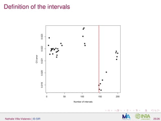
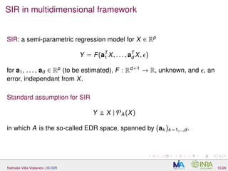
The document discusses interpretable sparse sliced inverse regression (IS-SIR) for functional data regression. It begins with background on using metamodels as proxies for computationally expensive agronomic models to understand relationships between climate inputs and plant outputs. SIR is presented as a semi-parametric regression technique that identifies relevant subspaces to predict outputs from functional inputs. The proposal involves combining SIR with automatic interval selection to point out interpretable predictor intervals. Simulations are discussed to evaluate the proposed method.


![A first case study: SUNFLO [Casadebaig et al., 2011]
Inputs: 5 daily time series (length: one year) and 8 phenotypes for different
sunflower types
Output: sunflower yield
Data: 1000 sunflower types × 190 climatic series (different places and
years) (n = 190 000) of variables in R5×183
× R8
Nathalie Villa-Vialaneix | IS-SIR 5/26](https://image.slidesharecdn.com/slides2016-04-08-bordeaux-160408131517/85/Interpretable-Sparse-Sliced-Inverse-Regression-for-digitized-functional-data-9-320.jpg)


![Related works (variable selection in FDA)
LASSO / L1
regularization in linear models
[Ferraty et al., 2010, Aneiros and Vieu, 2014] (isolated evaluation
points), [Matsui and Konishi, 2011] (selects elements of an expansion
basis), [James et al., 2009] (sparsity on derivatives: piecewise
constant predictors)
[Fraiman et al., 2015] (blinding approach useable for various
problems: PCA, regression...)
[Gregorutti et al., 2015] adaptation of the importance of variables in
random forest for groups of variables
Nathalie Villa-Vialaneix | IS-SIR 8/26](https://image.slidesharecdn.com/slides2016-04-08-bordeaux-160408131517/85/Interpretable-Sparse-Sliced-Inverse-Regression-for-digitized-functional-data-15-320.jpg)
![Related works (variable selection in FDA)
LASSO / L1
regularization in linear models
[Ferraty et al., 2010, Aneiros and Vieu, 2014] (isolated evaluation
points), [Matsui and Konishi, 2011] (selects elements of an expansion
basis), [James et al., 2009] (sparsity on derivatives: piecewise
constant predictors)
[Fraiman et al., 2015] (blinding approach useable for various
problems: PCA, regression...)
[Gregorutti et al., 2015] adaptation of the importance of variables in
random forest for groups of variables
Our proposal: a semi-parametric (not entirely linear) model which selects
relevant intervals combined with an automatic procedure to define the
intervals.
Nathalie Villa-Vialaneix | IS-SIR 8/26](https://image.slidesharecdn.com/slides2016-04-08-bordeaux-160408131517/85/Interpretable-Sparse-Sliced-Inverse-Regression-for-digitized-functional-data-16-320.jpg)

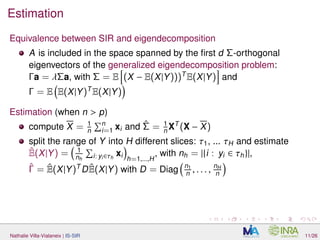
![Equivalent formulations
SIR as a regression problem [Li and Yin, 2008] shows that SIR is
equivalent to the (double) minimization of
E(A, C) =
H
h=1
ˆph Xh − X − ˆΣACh
2
for Xh = 1
nh i: yi∈τh
, A a (p × d)-matrix and C a vector in Rd
.
Nathalie Villa-Vialaneix | IS-SIR 12/26](https://image.slidesharecdn.com/slides2016-04-08-bordeaux-160408131517/85/Interpretable-Sparse-Sliced-Inverse-Regression-for-digitized-functional-data-24-320.jpg)
![Equivalent formulations
SIR as a regression problem [Li and Yin, 2008] shows that SIR is
equivalent to the (double) minimization of
E(A, C) =
H
h=1
ˆph Xh − X − ˆΣACh
2
for Xh = 1
nh i: yi∈τh
, A a (p × d)-matrix and C a vector in Rd
.
Rk: Given A, C is obtained as the solution of an ordinary least square
problem...
Nathalie Villa-Vialaneix | IS-SIR 12/26](https://image.slidesharecdn.com/slides2016-04-08-bordeaux-160408131517/85/Interpretable-Sparse-Sliced-Inverse-Regression-for-digitized-functional-data-25-320.jpg)
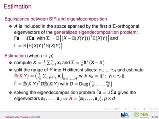
![Equivalent formulations
SIR as a regression problem [Li and Yin, 2008] shows that SIR is
equivalent to the (double) minimization of
E(A, C) =
H
h=1
ˆph Xh − X − ˆΣACh
2
for Xh = 1
nh i: yi∈τh
, A a (p × d)-matrix and C a vector in Rd
.
Rk: Given A, C is obtained as the solution of an ordinary least square
problem...
SIR as a Canonical Correlation problem [Li and Nachtsheim, 2008]
shows that SIR rewrites as the double optimisation problem
maxaj,φ Cor(φ(Y), aT
j
X), where φ is any function R → R and (aj)j are
Σ-orthonormal.
Nathalie Villa-Vialaneix | IS-SIR 12/26](https://image.slidesharecdn.com/slides2016-04-08-bordeaux-160408131517/85/Interpretable-Sparse-Sliced-Inverse-Regression-for-digitized-functional-data-26-320.jpg)
![Equivalent formulations
SIR as a regression problem [Li and Yin, 2008] shows that SIR is
equivalent to the (double) minimization of
E(A, C) =
H
h=1
ˆph Xh − X − ˆΣACh
2
for Xh = 1
nh i: yi∈τh
, A a (p × d)-matrix and C a vector in Rd
.
Rk: Given A, C is obtained as the solution of an ordinary least square
problem...
SIR as a Canonical Correlation problem [Li and Nachtsheim, 2008]
shows that SIR rewrites as the double optimisation problem
maxaj,φ Cor(φ(Y), aT
j
X), where φ is any function R → R and (aj)j are
Σ-orthonormal.
Rk: The solution is shown to satisfy φ(y) = aT
j
E(X|Y = y) and aj is
also obtained as the solution of the mean square error problem:
min
aj
E φ(Y) − aT
j X
2
Nathalie Villa-Vialaneix | IS-SIR 12/26](https://image.slidesharecdn.com/slides2016-04-08-bordeaux-160408131517/85/Interpretable-Sparse-Sliced-Inverse-Regression-for-digitized-functional-data-27-320.jpg)
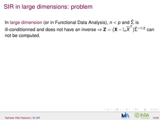
![SIR in large dimensions: problem
In large dimension (or in Functional Data Analysis), n < p and ˆΣ is
ill-conditionned and does not have an inverse ⇒ Z = (X − InX
T
)ˆΣ−1/2
can
not be computed.
Different solutions have been proposed in the litterature based on:
prior dimension reduction (e.g., PCA) [Ferré and Yao, 2003] (in the
framework of FDA)
regularization (ridge...) [Li and Yin, 2008, Bernard-Michel et al., 2008]
sparse SIR
[Li and Yin, 2008, Li and Nachtsheim, 2008, Ni et al., 2005]
Nathalie Villa-Vialaneix | IS-SIR 13/26](https://image.slidesharecdn.com/slides2016-04-08-bordeaux-160408131517/85/Interpretable-Sparse-Sliced-Inverse-Regression-for-digitized-functional-data-29-320.jpg)
![SIR in large dimensions: ridge penalty / L2-regularization
of ˆΣ
Following [Li and Yin, 2008] which shows that SIR is equivalent to the
minimization of
E2(A, C) =
H
h=1
ˆph Xh − X − ˆΣACh
2
,
Nathalie Villa-Vialaneix | IS-SIR 14/26](https://image.slidesharecdn.com/slides2016-04-08-bordeaux-160408131517/85/Interpretable-Sparse-Sliced-Inverse-Regression-for-digitized-functional-data-30-320.jpg)
![SIR in large dimensions: ridge penalty / L2-regularization
of ˆΣ
Following [Li and Yin, 2008] which shows that SIR is equivalent to the
minimization of
E2(A, C) =
H
h=1
ˆph Xh − X − ˆΣACh
2
+µ2
H
h=1
ˆph ACh
2
,
[Bernard-Michel et al., 2008] propose to penalize by a ridge penalty in a
high dimensional setting.
Nathalie Villa-Vialaneix | IS-SIR 14/26](https://image.slidesharecdn.com/slides2016-04-08-bordeaux-160408131517/85/Interpretable-Sparse-Sliced-Inverse-Regression-for-digitized-functional-data-31-320.jpg)
![SIR in large dimensions: ridge penalty / L2-regularization
of ˆΣ
Following [Li and Yin, 2008] which shows that SIR is equivalent to the
minimization of
E2(A, C) =
H
h=1
ˆph Xh − X − ˆΣACh
2
+µ2
H
h=1
ˆph ACh
2
,
[Bernard-Michel et al., 2008] propose to penalize by a ridge penalty in a
high dimensional setting.
They also show that this problem is equivalent to finding the eigenvectors
of the generalized eigenvalue problem
ˆΓa = λ ˆΣ + µ2Ip a.
Nathalie Villa-Vialaneix | IS-SIR 14/26](https://image.slidesharecdn.com/slides2016-04-08-bordeaux-160408131517/85/Interpretable-Sparse-Sliced-Inverse-Regression-for-digitized-functional-data-32-320.jpg)
![SIR in large dimensions: sparse versions
Specific issue to introduce sparsity in SIR
sparsity on a multiple-index model. Most authors use shrinkage
approaches.
First version: sparse penalization of the ridge solution
If (ˆA, ˆC) are the solutions of the ridge SIR as described in the previous
slide, [Ni et al., 2005, Li and Yin, 2008] propose to shrink this solution by
minimizing
Es,1(α) =
H
h=1
ˆph Xh − X − ˆΣDiag(α)ˆA ˆCh
2
+ µ1 α L1
(regression formulation of SIR)
Nathalie Villa-Vialaneix | IS-SIR 15/26](https://image.slidesharecdn.com/slides2016-04-08-bordeaux-160408131517/85/Interpretable-Sparse-Sliced-Inverse-Regression-for-digitized-functional-data-33-320.jpg)
![SIR in large dimensions: sparse versions
Specific issue to introduce sparsity in SIR
sparsity on a multiple-index model. Most authors use shrinkage
approaches.
Second version: [Li and Nachtsheim, 2008] derive the sparse optimization
problem from the correlation formulation of SIR:
min
as
j
n
i=1
Pˆaj
(X|yi) − (as
j )T
xi
2
+ µ1,j as
j L1
,
in which Pˆaj
is the projection of ˆE(X|Y = yi) = Xh onto the space spanned
by the solution of the ridge problem.
Nathalie Villa-Vialaneix | IS-SIR 15/26](https://image.slidesharecdn.com/slides2016-04-08-bordeaux-160408131517/85/Interpretable-Sparse-Sliced-Inverse-Regression-for-digitized-functional-data-34-320.jpg)
![Characteristics of the different approaches and possible
extensions
[Li and Yin, 2008] [Li and Nachtsheim, 2008]
sparsity on shrinkage coefficients estimates
nb optimization pb 1 d
sparsity common to all dims specific to each dim
Nathalie Villa-Vialaneix | IS-SIR 16/26](https://image.slidesharecdn.com/slides2016-04-08-bordeaux-160408131517/85/Interpretable-Sparse-Sliced-Inverse-Regression-for-digitized-functional-data-35-320.jpg)
![Characteristics of the different approaches and possible
extensions
[Li and Yin, 2008] [Li and Nachtsheim, 2008]
sparsity on shrinkage coefficients estimates
nb optimization pb 1 d
sparsity common to all dims specific to each dim
Extension to block-sparse SIR (like in PCA)?
Nathalie Villa-Vialaneix | IS-SIR 16/26](https://image.slidesharecdn.com/slides2016-04-08-bordeaux-160408131517/85/Interpretable-Sparse-Sliced-Inverse-Regression-for-digitized-functional-data-36-320.jpg)


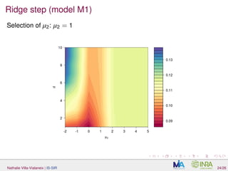
![Parameter estimation
H (number of slices): usually, SIR is known to be not very sensitive to
the number of slices (> d + 1). We took H = 10 (i.e., 10/30
observations per slice);
µ2 and d (ridge estimate ˆA):
L-fold CV for µ2 (for a d0 large enough) Note that GCV as described in
[Li and Yin, 2008] can not be used since the current version of the L2
penalty involves the use of an estimate of Σ−1
.
Nathalie Villa-Vialaneix | IS-SIR 20/26](https://image.slidesharecdn.com/slides2016-04-08-bordeaux-160408131517/85/Interpretable-Sparse-Sliced-Inverse-Regression-for-digitized-functional-data-43-320.jpg)
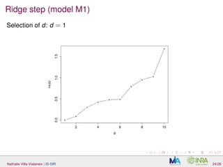
![Parameter estimation
H (number of slices): usually, SIR is known to be not very sensitive to
the number of slices (> d + 1). We took H = 10 (i.e., 10/30
observations per slice);
µ2 and d (ridge estimate ˆA):
L-fold CV for µ2 (for a d0 large enough)
using again L-fold CV, ∀ d = 1, . . . , d0, an estimate of
R(d) = d − E Tr Πd
ˆΠd ,
in which Πd and ˆΠd are the projector onto the first d dimensions of the
EDR space and its estimate, is derived similarly as in
[Liquet and Saracco, 2012]. The evolution of ˆR(d) versus d is studied
to select a relevant d.
Nathalie Villa-Vialaneix | IS-SIR 20/26](https://image.slidesharecdn.com/slides2016-04-08-bordeaux-160408131517/85/Interpretable-Sparse-Sliced-Inverse-Regression-for-digitized-functional-data-44-320.jpg)
![Parameter estimation
H (number of slices): usually, SIR is known to be not very sensitive to
the number of slices (> d + 1). We took H = 10 (i.e., 10/30
observations per slice);
µ2 and d (ridge estimate ˆA):
L-fold CV for µ2 (for a d0 large enough)
using again L-fold CV, ∀ d = 1, . . . , d0, an estimate of
R(d) = d − E Tr Πd
ˆΠd ,
in which Πd and ˆΠd are the projector onto the first d dimensions of the
EDR space and its estimate, is derived similarly as in
[Liquet and Saracco, 2012]. The evolution of ˆR(d) versus d is studied
to select a relevant d.
µ1 (LASSO) glmnet is used, in which µ1 is selected by CV along the
regularization path.
Nathalie Villa-Vialaneix | IS-SIR 20/26](https://image.slidesharecdn.com/slides2016-04-08-bordeaux-160408131517/85/Interpretable-Sparse-Sliced-Inverse-Regression-for-digitized-functional-data-45-320.jpg)


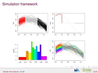
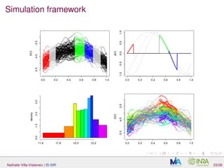
![Simulation framework
Data generated with:
Y = d
j=1 log X, aj with X(t) = Z(t) + in which Z is a Gaussian
process with mean µ(t) = −5 + 4t − 4t2
and the Matern 3/2
covariance function with parameters σ = 0.1 and θ = 0.2/
√
3, is a
centered Gaussian variable independant of Z, with standard deviation
0.1.;
aj = sin
t(2+j)π
2 −
(j−1)π
3 IIj
(t)
two models: (M1), d = 1, I1 = [0.2, 0.4]. For (M2), d = 3 and
I1 = [0, 0.1], I2 = [0.5, 0.65] and I3 = [0.65, 0.78].
Nathalie Villa-Vialaneix | IS-SIR 23/26](https://image.slidesharecdn.com/slides2016-04-08-bordeaux-160408131517/85/Interpretable-Sparse-Sliced-Inverse-Regression-for-digitized-functional-data-53-320.jpg)