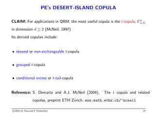
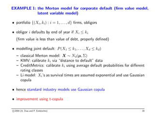
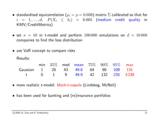
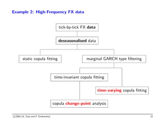
The document discusses quantitative risk management, focusing on the applications and implications of copulas in financial risk analysis. It introduces fundamental theorems, regulatory frameworks, and common misconceptions regarding risk management tools, emphasizing the importance of understanding dependencies in risk assessment. Examples include modeling credit risk using copulas and stress testing within a multivariate framework.


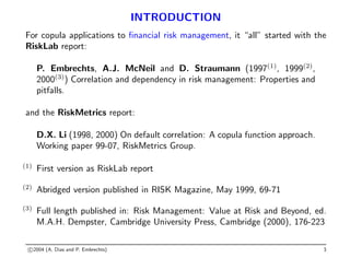


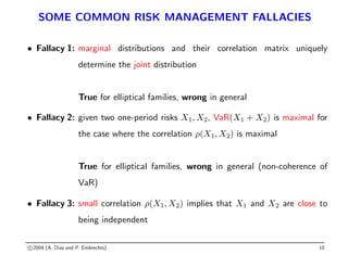
![THE TAIL LIMIT COPULA
Lower Tail Limit Copula Convergence Theorem: Let C be an exchangeable
copula such that C(v, v) 0 for all v 0. Assume that there is a strictly
increasing continuous function K : [0, ∞) → [0, ∞) such that
lim
v→0
C(vx, v)
C(v, v)
= K(x), x ∈ [0, ∞).
Then there is η 0 such that K(x) = xη
K(1/x) for all (0, ∞). Moreover, for
all (u1, u2) ∈ (0, 1]2
Clo
0 (u1, u2) = G(K−1
(u1), K−1
(u2)),
where G(x1, x2) := xη
2K(x1/x2) for (x1, x2) ∈ (0, 1]2
, G := 0 on [0, 1]2
(0, 1]2
and Clo
0 denotes the lower tail limit copula
Observation: The function K(x) fully determines the tail limit copula
c 2004 (A. Dias and P. Embrechts) 18](https://image.slidesharecdn.com/quebec-230601221833-961168c2/85/quebec-pdf-19-320.jpg)
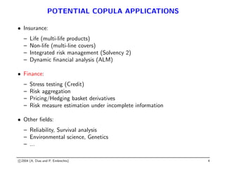
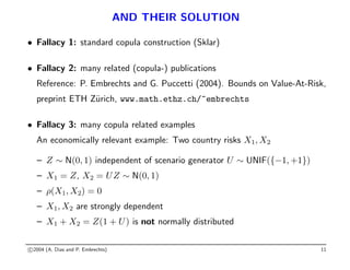
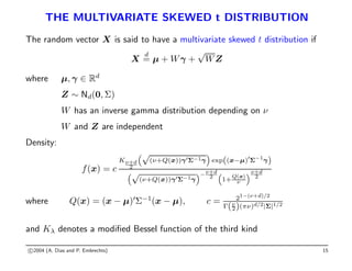
![THE t LOWER TAIL LIMIT COPULA
For the bivariate t-copula Ct
ν,ρ with tail dependence coefficient λ we have for
the t-LTL copula that
K(x) =
xtν+1
−(x1/ν
−ρ)
√
1−ρ2
√
ν + 1
+ tν+1
−(x−1/ν
−ρ)
√
1−ρ2
√
ν + 1
λ
with x ∈ [0, 1], whereas for the Clayton-LTL copula, with parameter θ,
K(x) = (x−θ
+ 1)/2
−1/θ
Important for pratice: “for any pair of parameter values ν and ρ the
K-function of the t-LTL copula may be very closely approximated by the K-
function of the Clayton copula for some value of θ” (S. Demarta and A.J.
McNeil (2004))
c 2004 (A. Dias and P. Embrechts) 19](https://image.slidesharecdn.com/quebec-230601221833-961168c2/85/quebec-pdf-20-320.jpg)

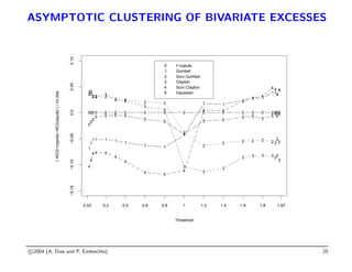
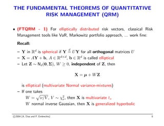
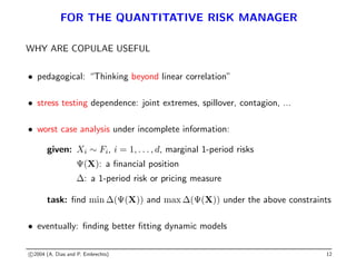
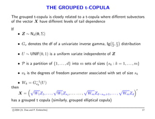
![ASYMPTOTIC CLUSTERING OF BIVARIATE EXCESSES
• Extreme tail dependence copula relative to a threshold t:
Ct(u, v) = P(U ≤ F−1
t (u), V ≤ F−1
t (v)|U ≤ t, V ≤ t)
with conditional distribution function
Ft(u) := P(U ≤ u|U ≤ t, V ≤ t), 0 ≤ u ≤ 1
• Archimedean copulae: there exists a continuous, strictly decreasing function
ψ : [0, 1] 7→ [0, ∞] with ψ(1) = 0, such that
C(u, v) = ψ[−1]
(ψ(u) + ψ(v))
• For “sufficiently regular” Archimedean copulae (Juri and Wüthrich (2002)):
lim
t→0+
Ct(u, v) = CClayton
α (u, v)
Juri, A. and M. Wüthrich (2002). Copula convergence theorems for tail events.
Insurance: Math. Econom., 30: 405–420
c 2004 (A. Dias and P. Embrechts) 24](https://image.slidesharecdn.com/quebec-230601221833-961168c2/85/quebec-pdf-25-320.jpg)