This document discusses time series forecasting techniques for multivariate and hierarchical time series data. It presents several cases involving energy consumption forecasting, sales forecasting, and freight transportation forecasting. For each case, it describes the time series data and components, discusses feature generation methods like nonparametric transformations and the Haar wavelet transform to extract features, and evaluates different forecasting models and their ability to generate consistent forecasts while respecting any hierarchical relationships in the data. The focus is on generating accurate forecasts while maintaining properties like consistency, minimizing errors, and handling complex time series structures.

1. Business intelligence III:
Feature generation and model selection
for multiscale time series forecasting
Vadim Strijov
Moscow Institute of Physics and Technology
AINL FRUCT
2016, 10 - 12 of November
1 / 68

2. Model selection for time series forecasting
The Internet of things is the world of networking devices (portables, vehicles, buildings)
embedded with sensors and software.
Environment and energy monitoring
Medical and health monitoring
Consumer support, sales monitoring
Urban management and manufacturing
2 / 68

3. Case 1. Energy consumption and price forecasting, 1-day ahead hourly
The components of multivariate time series with periodicity
Time series:
energy price,
consumption,
daytime,
temperature,
humidity,
wind force,
holiday schedule.
Periodicity:
one year seasons
(temperature,
daytime),
one week,
one day (working
day, week-end),
a holiday,
aperiodic events.
3 / 68

4. Energy consumption one-week forecast for each hour
4 / 68

5. The autoregressive matrix, five weeks
2 4 6 8 10 12 14 16 18 20 22 24
5
10
15
20
25
30
35
40
Hours
Days
5 / 68

6. The autoregressive matrix and the linear model
X∗
(m+1)×(n+1)
=










ˆsT sT−1 . . . sT−κ+1
s(m−1)κ s(m−1)κ−1 . . . s(m−2)κ+1
. . . . . . . . . . . .
snκ snκ−1 . . . sn(κ−1)+1
. . . . . . . . . . . .
sκ sκ−1 . . . s1










=


ˆsT
1×1
xm+1
1×n
y
m×1
X
m×n

 .
In terms of linear regression:
ˆy = f(X, w) = Xw,
ˆym+1 = ˆsT = xm+1, ˆw .
6 / 68

7. The one-day forecast: expected error is 3.1% working day, 3.7% week-end
5 10 15 20
1.5
1.6
1.7
1.8
1.9
2
2.1
2.2
2.3
x 10
4
Hours
Value
History
Forecast
The model ˆy = f(X, w) could be a linear model, neural network, deep NN, SVN, . . .
7 / 68

8. Structure of energy consumption
8 / 68

9. Similarity of daily consumption
9 / 68

10. Sunrise bias: one-year daytime and consumption
10 / 68

11. Biased and original daytime to fit consumption over years
11 / 68

12. One-hour line, day-by-day during a year: autoregressive analysis
12 / 68

13. Daily similarity
13 / 68

14. The model performance criteria and forecast errors
Stability:
the error does not change significantly following small changes in time series,
the distribution of the model parameters does not change.
Complexity:
the number of parameters (elements in superposition) is minimal,
the minimum description length principle holds the William Ockham’s rule.
Error: the residue εj = ˆyj − yj for
mean absolute error and (symmetric) mean absolute percent error
RSS =
r
j=1
ε2
j , MAPE =
1
r
r
j=1
|εj |
|yj |
, sMAPE =
1
r
r
j=1
2|εj |
|ˆyj + yj |
.
14 / 68

15. Design matrix
Forecast is a mapping from p-dimensional objects space to r-dimensional answers
space.
X∗
=
x
1×n
y
1×r
X
m×n
Y
m×r
15 / 68

16. Rolling validation
Z =







. . . . . .
xval,k
1×n
yval,k
1×r
Xtrain,k
mmin×n
Ytrain,k
mmin×r
. . . . . .









k
The rolling validation procedure
1) construct the validation vector x∗
val,k for time series of the length ∆tr as the first
row of the design matrix Z,
2) construct the rest rows of the design matrix Z for the time after tk and present it as
3) optimize model parameters w using Xtrain,k, Ytrain,k and compute
residues εk = yval,k − f(xvalk
, w) and MAPE,
4) increase k and repeat.
16 / 68

17. Case 2. Sales planning: to forecast the goods consumption
Retailers’ daily routines:
custom inventory,
calculation of optimal insurance stocks,
consumer demand forecasting.
There given historical time series of the volume off-takes: foodstuff.
Let the time series be homoscedastic: its variance is time-constant.
Minimizing the loss function one must forecast the next sample.
17 / 68

18. Custom inventory
18 / 68

19. Excessive forecast and insufficient forecast lead to loss
19 / 68

20. The performance criterion is minimum loss of money
Error functions: quadratic, linear, asymmetric.
20 / 68

21. The time series of residues and its histogram
There given historgam
H = {Xi , gi }m
i=1
and loss function
L = L(Z, X).
The optimal forecast is
˜X = arg min
Z∈{X1...Xm}
m
i=1
gi L(Z, Xi )
of this convolution.
21 / 68

22. Candies: the seasonality and trend weekly over three years
22 / 68

23. Beverage: the week periodicity daily over four weeks
23 / 68

24. Sparkling wine: holidays weekly over three years
24 / 68

25. Promotional actions
25 / 68

26. Promotional profile extraction
Hypothesis: the shape of the profile (excluding the profile parameters) does not
depend of duration of the action.
Problem: to forecast the customer demand during the promotional action.
26 / 68

27. Forecast the residues to boost performance
1. Model f forecasts n(g) history ends ˆxf
t , ..., ˆxf
t−n(g)+1 for one sample.
2. Compute n(g) residues ˆεt, ..., ˆεt−n(g)+1 as ˆεt−k = xt−k − ˆxf
t−k.
3. Function g forecasts residues ˆεt+i ahead max(i) time-ticks.
4. Combine forecasts ˆxf ,g
t+i = ˆxf
t+i + ˆεt+i computing f for each sample ˆxf
t+i .
27 / 68

28. Case 3. Forecasting volumes of Russian railways freight transportation
Keep a hierarchical structure of time series without loosing performance
Forecast with hierarchical aggregation of
types of freight in
stations, regions, and roads,
for a day, week, month, and quarter,
counting all combinations above.
Satisfy the conditions:
minimize error,
incorporate important external factors,
respect hierarchical structure,
do not exceed physical bounds of forecast values. 28 / 68

29. The railroad map counts ∼ 78 regions, ∼ 4000 stations, and ∼ 100 rail-yards
29 / 68

30. Independent forecasts might be inconsistent with aggregated ones
Time
50 100 150 200
Timeseries
-0.4
-0.2
0
0.2
0.4
30 / 68

31. Hierarchical data χ, independent forecasts ˆχ and reconciliated forecasts ˆϕ
χt =






xt(:, :)
. . .
xt(n, 1)
. . .
xt(n, m)






, ˆχ =






ˆx(:, :)
. . .
ˆx(n, 1)
. . .
ˆx(n, m)






, ˆϕ =






ˆy(:, :)
. . .
ˆy(n, 1)
. . .
ˆy(n, m)






.
Consistency condition Sχt = 0, t = 1, . . . , T, where the
link matrix S of size (2 + n + m) × (1 + n + m + nm) has the form
S =











−1 1 . . . 1 0 . . . 0 0 0 . . . 0 . . . 0 0 . . . 0
−1 0 . . . 0 1 . . . 1 0 0 . . . 0 . . . 0 0 . . . 0
0 −1 . . . 0 0 . . . 0 1 1 . . . 1 . . . 0 0 . . . 0
. . . . . . . . . . . . . . .
0 0 . . . −1 0 . . . 0 0 0 . . . 0 . . . 1 1 . . . 1
0 0 . . . 0 −1 . . . 0 1 0 . . . 0 . . . 1 0 . . . 0
. . . . . . . . . . . . . . .
0 0 . . . 0 0 . . . −1 0 0 . . . 1 . . . 0 0 . . . 1











.
The regions
xt(:, :) =
n
i=1
xt(i, :);
The freights
xt(:, :) =
m
j=1
xt(:, j);
Freights given a region
xt(i, :) =
m
j=1
xt(i, j),
i = 1, . . . n;
Regions given a freight
xt(:, j) =
n
i=1
xt(i, j),
j = 1, . . . m;
t = 1, . . . , T.
31 / 68

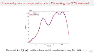
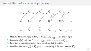
32. Performance of independent and reconciliated forecasts
There given link matrix S, admissible sets A, B
and independent forecasts ˆχ ∈ A, ˆχ ∈ B
to make reconciliated forecast ˆϕ subject to
consistency ˆϕ ∈ A, A = {χ ∈ Rd
| Sχ = 0},
physical limitations ˆϕ ∈ B,
precision lh(χT+1, ˆϕ) ≤ lh(χT+1, ˆχ) for any
hierarchical data χT+1 ∈ A ∩ B.
Theorem [Maria Stenina, 2014]
Given listed conditions, the projection vector
ˆϕ = χproj = arg min
χ∈A∩B
lh(χ, ˆχ)
is guaranteed to satisfy the requirements of
consistency, physical limitations and precision.
The solution of the optimization
problem ˆϕ = arg min
χ∈A∩B
χ − ˆχ 2
2
demonstrates decrease in loss for all
control samples.
0 20 40 60 80 100
−6
−5
−4
−3
−2
−1
0
x 10
6
Control point
Lt
Lt = χt − ˆϕ 2
2 − χt − ˆχ 2
2
32 / 68

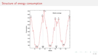
33. Case 4. Internet of things, multiscale dataset for vector forecasting
Days
Energy
Max T.
Min T.
Precipitation
Wind
Humidity
Solar
Energy
Solar
τ′
τ
ti ti+1 t′
i = iτ′ t′
i+1
Each real-valued time series s = [s1, . . . , si , . . . , sT ], si = s(ti ), 0 ≤ ti ≤ tmax
is a sequence of observations of some real-valued signal s(t) with its own sampling rate τ.
33 / 68

34. To boost the forecast quality include external variables
34 / 68

35. Generate features with nonparametric transformation functions
Univariate
Formula Output dimension
√
x 1
x
√
x 1
arctan x 1
ln x 1
x ln x 1
Bivariate
Plus x1 + x2
Minus x1 − x2
Product x1 · x2
Division x1
x2
x1
√
x2
x1 ln x2
35 / 68

36. Nonparametric aggregation: sample statistics
Nonparametric transformations include basic data statistics:
Sum or average value of each row xi , i = 1, . . . , m:
φi =
n
j=1
xij , or φi =
1
n
n
j=1
xij .
Min and max values: φi = minj xij , φi = maxj xij .
Standard deviation:
φi =
1
n − 1
n
j=1
(xij − mean(xi ))2.
Data quantiles: φi = [X1, . . . , XK ], where
n
j=1
[Xk−1 < xij ≤ Xk] =
1
K
, for k = 1, . . . , K.
36 / 68

37. Nonparametric transformations: Haar’s transform
Applying Haar’s transform produces multiscale representations of the same data.
Assume that n = 2K
and init φ
(0)
i,j
= φ
(0)
i,j
= xij for j = 1, . . . , n.
To obtain coarse-graining and fine-graining of the input feature vector xi , for
k = 1, . . . , K repeat:
data averaging step
φ
(k)
i,j =
φ
(k−1)
i,2j−1 + φ
(k−1)
i,2j
2
, j = 1, . . . ,
n
2k
,
and data differencing step
φ
(k)
i,j =
φ
(k−1)
i,2j − φ
(k−1)
i,2j−1
2
, j = 1, . . . ,
n
2k
.
The resulting multiscale feature vectors are φi = [φ
(1)
i
, . . . , φ
(K)
i
] and φi = [φ
(1)
i
, . . . , φ
(K)
i
].
37 / 68

38. Monotone functions
By grow rate
Function name Formula Constraints
Linear w1x + w0
Exponential rate exp(w1x + w0) w1 > 0
Polynomial rate exp(w1 ln x + w0) w1 > 1
Sublinear
polynomial rate
exp(w1 ln x + w0) 0 < w1 < 1
Logarithmic rate w1 ln x + w0 w1 > 0
Slow convergence w0 + w1/x w1 = 0
Fast convergence w0 + w1 · exp(−x) w1 = 0
Other
Soft ReLu ln(1 + ex )
Sigmoid 1/(w0 + exp(−w1x)) w1 > 0
Softmax 1/(1 + exp(−x))
Hiberbolic tangent tanh(x)
softsign |x|
1+|x| 38 / 68

39. Collection of parametric transformation functions
Function
name
Formula Output
dim.
Num.
of args
Num.
of pars
Add constant x + w 1 1 1
Quadratic w2x2 + w1x + w0 1 1 3
Cubic w3x3 + w2x2 + w1x + w0 1 1 4
Logarithmic
sigmoid
1/(w0 + exp(−w1x)) 1 1 2
Exponent exp x 1 1 0
Normal 1
w1
√
2π
exp (x−w2)2
2w2
1
1 1 2
Multiply by
constant
x · w 1 1 1
Monomial w1xw2 1 1 2
Weibull-2 w1w2xw2−1 exp −w1xw2 1 1 2
Weibull-3 w1w2xw2−1 exp −w1(x − w3)w2 1 1 3
. . . . . . . . . . . . . . . 39 / 68

40. Parametric transformations
Optimization of the transformation function parameters b is iterative:
1. Fix the vector ˆb, collected over all the primitive functions {g}, which generate
features φ:
ˆw = arg min S w|f(w, x), y , where φ(ˆb, s) ⊆ x.
2. Optimize transformation parameters ˆb given model parameters ˆw
ˆb = arg min S b|f(ˆw, x), y .
Repeat these steps until vectors ˆw, ˆb converge.
40 / 68

41. Markup the time series, two types of marks: Up and Down
41 / 68

42. Parameters of the local models
More feature generation options:
Parameters of SSA approximation of the time series x(q).
Parameters of the FFT of each x(q).
Parameters of polynomial/spline approximation of each x(q).
42 / 68

43. Parameters of the local models: SSA
For the time series s construct the Hankel matrix with a period k and shift p, so that
for s = [s1, . . . , sT ] the matrix
H∗
=





sT . . . sT−k+1
...
...
...
sk+p . . . s1+p
sk . . . s1





, where 1 p k.
Reconstruct the regression to the first column of the matrix H∗ = [h, H] and denote its
least square parameters as the feature vector
φ(s) = arg min h − Hφ 2
2.
For the orignal feature vector x = [x(1), . . . , x(Q)] use the parameters φ(x(q)),
q = 1, . . . , Q as the features.
43 / 68

44. SSA: principal components
Compute the SVD of covariance matrix of H
1
N
H
T
H = VΛV
T
, Λ = diag(λ1, . . . , λN)
and find the principal components yj = Hvj .
−5 0 5
−6
−4
−2
0
2
4
6
8
Principal component, y1
Principalcomponent,y2
44 / 68

45. Models and features
Models:
Baseline method: ˆsi = si−1.
Multivariate linear regression (MLR) with l2-regularization. Regularization coefficient: 2
SVR with multiple output. Kernel type: RBF, p1: 2, p2: 0, γ: 0.5, λ: 4.
Feed-forward ANN with single hidden layer, size: 25
Random forest (RF). Number of trees: 25 , number of variables for each decision split: 48.
Feature combinations:
History: the standard regression-based forecast with no additional features.
SSA, Cubic, Conv, Centroids, NW: history + a particular feature.
All: all of the above, with no feature selection.
PCA and NPCA: all generation strategies with feature selection.
45 / 68

46. Feature analysis
H
istory
SSA
Cubic
ConvCentroids
N
W
A
ll
PCA
N
PCA
MLR
MSVR
RF
ANN
0
0.05
0.1
0.15
0.2
0.25
0.3
0.35
0.4
0.45
0.5
Test subset MAPE
Ratio of times each combination of model and feature performed best for at least one
of the time series (7) or error functions (6), all (6) data sets (6 × 7 × 6 = 252 cases).
46 / 68

47. Best models
Energy
M
ax
T.
M
in
T.Precipitation
W
ind
H
um
idity
Solar
ANNConv
MLRHistory
MSVRSSA
RFCubic
0
0.1
0.2
0.3
0.4
0.5
0.6
0.7
0.8
Test subset residues
Energy
M
ax
T.
M
in
T.Precipitation
W
ind
H
um
idity
Solar
MLRHistory
MSVRSSA
RFCubic
0
0.1
0.2
0.3
0.4
0.5
0.6
0.7
0.8
0.9
1
Standard deviations of test subset residues
47 / 68

48. Case 5. Classification of human physical activity with mobile devices
3D-projection of acceleration time series to spatial axis
x = {accx (t); accy (t); accz(t)}n
t=1 → y ∈ RS
.
Slow walking
0 1 2 3 4 5
−0.5
0
0.5
1
1.5
2
Time t, s
Acceleration,x,y,z
Jogging
0 1 2 3 4
−1
0
1
2
3
4
Time t, sAcceleration,x,y,z 48 / 68

49. Local transformations for deep learning neural network
Model f = a(hN(. . . h1(x)))(w) contains autoencoders hk and softmax classifier a:
f(w, x) =
exp(a(x))
j exp(aj (x))
, a(x) = W
T
2 tanh(W
T
1 x), hk(x) = σ(Wkx + bk),
where w minimizes the error function.
Feature generation by local transformations:
parameters of SSA approximation of the time series x,
FFT of x,
parameters of polynomial/spline approximation,
could reduce complexity this model down to complexity of logistic regression.
49 / 68

50. Parameters of the local models: SSA
For time series s construct the Hankel matrix with
a period k and shift p, so that for s = [s1, . . . , sT ]
the matrix
H∗
=





sT . . . sT−k+1
...
...
...
sk+2 . . . s2
sk . . . s1





.
−5 0 5
−6
−4
−2
0
2
4
6
8
Principal component, y1
Principalcomponent,y2
Reconstruct the regression to the first column of the matrix H∗ = [h, H] and denote its
least square parameters as the feature vector
φ(s) = arg min h − Hφ 2
2.
For the original feature vector x = [x(1), . . . , x(Q)] use the parameters φ(x) as an item.
50 / 68

51. Human gate detection with time series segmentation
Find dissection of the trajectory of principal components yj = Hvj , where H is the
Hankel matrix and vj are its eigenvectors:
1
N
H
T
H = VΛV
T
, Λ = diag(λ1, . . . , λN).
51 / 68

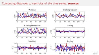
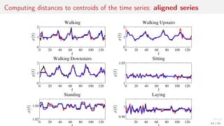
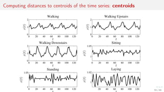
52. Metric features: distances to the centroids of local clusters
Apply kernel trick to the time series.
1. For objects xi from X compute k-mean centroids c.
2. Use distance function ρ to combine feature vector
φi = [ρ(c1, xi ), . . . , ρ(cp, xi )] ∈ Rp
+.
52 / 68

53. Computing distances to centroids of the time series: sources
0 20 40 60 80 100 120
0
1
2
Walking
t
x(t)
0 20 40 60 80 100 120
0
1
2
Walking Upstairs
t
x(t)
0 20 40 60 80 100 120
0
1
2
Walking Downstairs
t
x(t)
0 20 40 60 80 100 120
0.98
1
1.02
Sitting
t
x(t)
0 20 40 60 80 100 120
1.03
1.04
1.05
Standing
x(t)
20 40 60 80 100 120
0.99
1
Laying
x(t)
53 / 68

54. Computing distances to centroids of the time series: aligned series
0 20 40 60 80 100 120
0
1
2
Walking
t
x(t)
0 20 40 60 80 100 120
0
1
2
Walking Upstairs
t
x(t)
0 20 40 60 80 100 120
0
1
2
Walking Downstairs
t
x(t)
0 20 40 60 80 100 120
1
1.05
Sitting
t
x(t)
0 20 40 60 80 100 120
1.02
1.04
Standing
x(t)
20 40 60 80 100 120
0.98
1
Laying
x(t)
54 / 68

55. Computing distances to centroids of the time series: centroids
0 20 40 60 80 100 120
0
1
2
Walking
t
x(t)
0 20 40 60 80 100 120
0
1
2
Walking Upstairs
t
x(t)
0 20 40 60 80 100 120
0
1
2
Walking Downstairs
t
x(t)
0 20 40 60 80 100 120
1
1.05
Sitting
t
x(t)
0 20 40 60 80 100 120
1
1.05
Standing
x(t)
20 40 60 80 100 120
1
1.02
Laying
x(t)
55 / 68

56. Performance of the human physical activities classification model
1 2 3 4 5 6 7 8 9 10 11 12
Class labels
0
5
10
15
20
Objectsnumber
99.5% 97.8%
98.7% 98.8% 97.5%100.0%99.4% 93.4% 97.0% 99.9% 99.4% 97.2%
Mean Accuracy: 0.9823
1) walk forward
2) walk left
3) walk right
4) go upstairs
5) go downstairs
6) run forward
7) jump up and down
8) sit and fidget
9) stand
10) sleep
11) elevator up
12) elevator down
56 / 68

57. Case 6. How many parameters must be used? Relations of 24 hourly models
5 10 15 20
2
4
6
8
10
12
14
16
18
20
22
Hours
Parameters
57 / 68

58. Selection of a stable set of features of restricted size
The sample contains multicollinear χ1, χ2 and noisy χ5, χ6 features, columns of the design
matrix X. We want to select two features from six.
Stability and accuracy for a fixed complexity
The solution: χ3, χ4is an orthogonal set of features minimizing the error function.
58 / 68

59. Multicollinear features and the forecast: possible configurations
Inadequate and correlated Adequate and random
Adequate and redundant Adequate and correlated
59 / 68

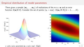
60. Model parameter values with regularization
Vector-function f = f(w, X) = [f (w, x1), . . . , f (w, xm)]T
∈ Ym.
0 2 4 6 8 10
−15
−10
−5
0
5
10
15
20
25
30
Regularization, τ
Parameters,w
S(w) = f(w, X) − y 2 + γ2 w 2
0 2 4 6 8
−2
−1
0
1
2
3
Parameters sum,
i
|wi|
Parameters,w
S(w) = f(w, X) − y 2, T(w) τ
60 / 68

61. Empirical distribution of model parameters
There given a sample {w1, . . . , wK } of realizations of the m.r.v. w and an error
function S(w|D, f). Consider the set of points {sk = exp −S(wk|D, f) |k = 1, . . . , K}.
0
0.2
0.4 0
0.2
0.4
0.02
0.04
0.06
0.08
w2w1
exp−S(w)
20 40 60 80 100
10
20
30
40
50
60
70
80
90
100
w1
w2
x- and y-axis: parameters w, z-axis: exp −S(w) . 61 / 68

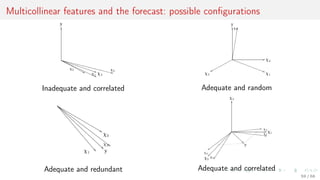
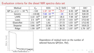
62. Minimize number of similar and maximize number of relevant features
Introduce a feature selection method QP(Sim, Rel) to solve the optimization problem
a∗
= arg min
a∈Bn
a
T
Qa − b
T
a,
where matrix Q ∈ Rn×n of pairwise similarities of features χi and χj is
Q = [qij ] = Sim(χi , χj ) =
Cov(χi , χj )
Var(χi )Var(χj )
and vector b ∈ Rn of feature relevances to the target is
b = [bi ] = Rel(χi ),
where elements bi equal absolute values of the sample correlation coefficient between
feature χi and the target vector y.
Number of correlated features Sim → min, number of correlated to the target Rel → max.
62 / 68

63. Evaluation criteria for the diesel NIR spectra data set
Method Cp RSS ln λ1
λn
SVD VIF BIC
QP (ρ, ρ) (τ = 10−9) −110 1.37 · 10−18 −25.7 6.43 · 106 548.38
Genetic −110.88 7.68 · 10−30 −24 8.13 · 105 534.19
LARS 3.22 · 1021 2.07 · 10−7 −28.3 7.94 · 107 529.47
Lasso 2.5 · 1028 1.61 −27.72 1.03 · 1021 1712.92
ElasticNet 2.51 · 1028 1.61 −27.72 1.03 · 1021 1712.92
Stepwise 3.66 · 1029 23.56 −36.78 1.94 · 1022 1919.23
Ridge 1.59 · 1028 1.02 −36.22 1.07 · 1022 1.79 · 103
Dependence of residual norm on the number of
selected features QP(Sim, Rel).
63 / 68

64. ECoG brain signals to forecast upper limbs’ movements
Neurotycho.org food-tracking dataset: 32 epidural electrodes
captures brain signals of the monkey (ECoG),
11 sensors track movements of the hand, contralateral to the
implant side,
experiment duration is 15 minutes,
the experimenter feeds the monkey ≈ 4.5 per minute,
ECoG and motion data were sampled at 1KHz and 120Hz,
respectively.
64 / 68

65. Weather forecasting and geo (spatio) temporal dataset
Monthly Ecosystem Respiration by M. Reichstein, GHG-Europe 65 / 68

66. Spatio temporal dataset, frequency versus time, given spatial position
Electric field measurement, the Van Allen probes by I. Zhelavskaya, Skoltech 66 / 68

67. Подробнее о вышеизложенных задачах
Авторегрессионное прогнозирование и выбор признаков
Катруца А., Стрижов В. Проблема мультиколлинеарности при выборе признаков в регрессионных задачах //
Информационные технологии, 2015, 1 : 8-18.
Нейчев Р.Г., Катруца А.М., Стрижов В. Выбор оптимального набора признаков из мультикоррелирующего множества в
задаче прогнозирования // Заводская лаборатория. Диагностика материалов, 2016, 3.
Мотренко А.П., Рудаков К.В., Стрижов В.В. Учет влияния экзогенных факторов при непараметрическом
прогнозировании временных рядов // Вестник Московского университета. Серия 15. Вычислительная математика и
кибернетика, 2016. A
Классификация временных рядов акселерометра
Ignatov A., Strijov V. Human activity recognition using quasiperiodic time series collected from a single triaxial accelerometer
// Multimedia Tools and Applications, 2015, 17.05.2015 : 1-14.
Motrenko A.P., Strijov V.V. Extracting fundamental periods to segment human motion time series // Journal of Biomedical
and Health Informatics, 2016.
Попова М.С., Стрижов В.В. Выбор оптимальной модели классификации физической активности по измерениям
акселерометра // Информатика и ее применения, 2015, 9(1) : 79-89.
Попова М. С., Стрижов В.В. Построение сетей глубокого обучения для классификации временных рядов // Системы и
средства информатики, 2015, 25(3) : 60-77.
Гончаров А.В., Стрижов В.В. Метрическая классификация временных рядов со взвешенным выравниванием
относительно центроидов классов // Информатика и ее применения, 2016, 2.
Согласование прогнозов иерархических временных рядов
Стенина М.М., Стрижов В.В. Согласование прогнозов при решении задач прогнозирования иерархических временных
рядов // Информатика и ее применения, 2015, 9(2) : 77-89.
Стенина М., Стрижов В. Согласование агрегированных и детализированных прогнозов при решении задач
непараметрического прогнозирования // Системы и средства информатики, 2014, 24(2) : 21-34.
67 / 68

68. Model selection for time series forecasting
Thanks to the Chair of Intelligent Systems, MIPT
Anastasia Motrenko
Mikhail Kuznetsov
Alexandr Aduenko
Arsentiy Kuzmin
Maria Stenina
Alexandr Katrutsa
Oleg Bakhteev
Maria Popova
Andrey Kulunchakov
Mikhail Karasikov
Radoslav Neychev
Alexey Goncharov
Roman Isachenko
Maria Vladimirova
http://machinelearning.ru
strijov@phystech.edu
68 / 68