![Frequency Estimation Techniques Peter J. Kootsookos [email_address]](https://image.slidesharecdn.com/compdspKootsookosFrequencyEstimation-122758273435-phpapp01/85/Frequency-Estimation-1-320.jpg)
![Frequency Estimation Techniques Peter J. Kootsookos [email_address]](https://image.slidesharecdn.com/compdspKootsookosFrequencyEstimation-122758273435-phpapp01/75/Frequency-Estimation-1-2048.jpg)
![Find the parameters A , , , and 2 in y(t) = A cos [ t- ) + )] + (t) where t = 0..T-1, T-1/2 and (t) is a noise with zero mean and variance 2 . is used to denote the vector [ A 2 ] T . Frequency Estimation Techniques What is frequency estimation?](https://image.slidesharecdn.com/compdspKootsookosFrequencyEstimation-122758273435-phpapp01/85/Frequency-Estimation-5-320.jpg)
![y(t) = A cos [ t- ) + )] + (t) What about A(t) ? Estimating A(t) is envelope estimation (AM demodulation). If the variation of A(t) is slow enough, the problem of estimating and estimating A(t) decouples. What about (t) ? This is the frequency tracking problem. What’s (t) ? Usually assumed additive, white, & Gaussian. Maximum likelihood technique depends on Gaussian assumption. Frequency Estimation Techniques What other problems are there?](https://image.slidesharecdn.com/compdspKootsookosFrequencyEstimation-122758273435-phpapp01/85/Frequency-Estimation-6-320.jpg)
![Amplitude-varying example: condition monitoring in rotating machinery. Frequency Estimation Techniques What other problems are there? [continued]](https://image.slidesharecdn.com/compdspKootsookosFrequencyEstimation-122758273435-phpapp01/85/Frequency-Estimation-7-320.jpg)
![Frequency tracking example: SONAR Frequency Estimation Techniques What other problems are there? [continued] Thanks to Barry Quinn & Ted Hannan for the plot from their book “The Estimation & Tracking of Frequency”.](https://image.slidesharecdn.com/compdspKootsookosFrequencyEstimation-122758273435-phpapp01/85/Frequency-Estimation-8-320.jpg)
![Frequency Estimation Techniques What other problems are there? [continued] Multi-harmonic frequency estimation y(t) = A m cos [m t- ) + m )] + (t) For periodic, but not sinusoidal, signals. Each component is harmonically related to the fundamental frequency. p m=1](https://image.slidesharecdn.com/compdspKootsookosFrequencyEstimation-122758273435-phpapp01/85/Frequency-Estimation-9-320.jpg)
![Frequency Estimation Techniques What other problems are there? [continued] Multi-tone frequency estimation y(t) = A m cos [ m t- ) + m )] + (t) Here, there are multiple frequency components with no relationship between the frequencies. p m=1](https://image.slidesharecdn.com/compdspKootsookosFrequencyEstimation-122758273435-phpapp01/85/Frequency-Estimation-10-320.jpg)
![The likelihood function for this problem, assuming that (t) is Gaussian is L( ) = 1/((2 ) T/2 |R |) exp(–( Y – Ŷ ( )) T R -1 ( Y – Ŷ ( ))/ 2) where R = The covariance matrix of the noise Y = [y(0) y(1) … y(T-1)] T Ŷ = [A cos( ) A cos( + ) … A cos( (T-1) + )] T Y is a vector of the date samples, and Ŷ is a vector of the modeled samples. Frequency Estimation Techniques The Maximum Likelihood Approach](https://image.slidesharecdn.com/compdspKootsookosFrequencyEstimation-122758273435-phpapp01/85/Frequency-Estimation-12-320.jpg)
![Two points to note: The functional form of the equation L( ) = 1/((2 ) T/2 |R |) exp(–( Y – Ŷ ( )) T R -1 ( Y – Ŷ ( ))/ 2) is determined by the Gaussian distribution of the noise. If the noise is white, then the covariance matrix R is just 2 I – a scaled identity matrix. Frequency Estimation Techniques The Maximum Likelihood Approach [continued]](https://image.slidesharecdn.com/compdspKootsookosFrequencyEstimation-122758273435-phpapp01/85/Frequency-Estimation-13-320.jpg)
![Often, it is easier to deal with the log-likelihood function: ℓ ( ) = –( Y – Ŷ ( ) ) T R -1 ( Y – Ŷ ( ) ) where the additive constant, and multiplying constant have been ignored as they do not affect the position of the peak (unless is zero or infinite). If the noise is also assumed to be white, the maximum likelihood problem looks like a least squares problem as maximizing the expression above is the same as minimizing ( Y – Ŷ ( ) ) T ( Y – Ŷ ( ) ) Frequency Estimation Techniques The Maximum Likelihood Approach [continued]](https://image.slidesharecdn.com/compdspKootsookosFrequencyEstimation-122758273435-phpapp01/85/Frequency-Estimation-14-320.jpg)
![Frequency Estimation Techniques The Maximum Likelihood Approach [continued] If the complex-valued signal model is used, then estimating is equivalent to maximizing the periodogram: P( ) = | y(t) exp(-i t) | 2 For the real-valued signal used here, this equivalence is only true as T tends to infinity. t=0 T-1](https://image.slidesharecdn.com/compdspKootsookosFrequencyEstimation-122758273435-phpapp01/85/Frequency-Estimation-15-320.jpg)
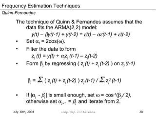
![The algorithm can be interpreted as finding the maximum of a smoothed periodogram. Frequency Estimation Techniques Quinn-Fernandes [continued]](https://image.slidesharecdn.com/compdspKootsookosFrequencyEstimation-122758273435-phpapp01/85/Frequency-Estimation-21-320.jpg)
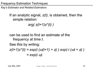
![Many signal processing problems already use “analytic” signals: communications systems with “in-phase” and “quadrature” components, for example. An analytic signal, exp(i-blah) , can be generated from a real-valued signal, cos(blah) , by use of the Hilbert transform: z(t) = y(t) + i H[ y(t) ] where H[.] is the Hilbert transform operation. Problems occur if the implementation of the Hilbert transform is poor. This can occur if, for example, too short an FIR filter is used. Frequency Estimation Techniques Associated Problems: Analytic Signal Generation](https://image.slidesharecdn.com/compdspKootsookosFrequencyEstimation-122758273435-phpapp01/85/Frequency-Estimation-24-320.jpg)
![Another approach is to FFT y(t) to obtain Y(k) . From Y(k) , form Z(k) = 2Y(k) for k = 1 to T/2 - 1 Y(k) for k = 0 0 for k = T/2 to T and then inverse FFT Z(k) to find z(t) . Unless Y(k) is interpolated, this can cause problems. Frequency Estimation Techniques Associated Problems: Analytic Signal Generation [continued] Makes sure the DC term is correct.](https://image.slidesharecdn.com/compdspKootsookosFrequencyEstimation-122758273435-phpapp01/85/Frequency-Estimation-25-320.jpg)
![If you know something about the signal (e.g. frequency range of interest), then use of a band-pass Hilbert transforming filter is a good option. See the paper by Andrew Reilly, Gordon Fraser & Boualem Boashash, “Analytic Signal Generation : Tips & Traps” IEEE Trans. on ASSP, vol 42(11), pp3241-3245 They suggest designing a real-coefficient low-pass filter with appropriate bandwidth using a good FIR filter algorithm (e.g. Remez). The designed filter is then modulated with a complex exponential of frequency f s /4. Frequency Estimation Techniques Associated Problems: Analytic Signal Generation [continued]](https://image.slidesharecdn.com/compdspKootsookosFrequencyEstimation-122758273435-phpapp01/85/Frequency-Estimation-26-320.jpg)
![What Kay did was to form an estimator = arg( w(t) z(t+1)z*(t) ) where the weights, w(t) , are chosen to minimize the mean square error. Kay found that, for very small noise w(t) = 6t(T-t) / (T(T 2 -1)) which is a parabolic window. Frequency Estimation Techniques Kay’s Estimator and Related Estimators [continued] ^ T-2 t=0](https://image.slidesharecdn.com/compdspKootsookosFrequencyEstimation-122758273435-phpapp01/85/Frequency-Estimation-28-320.jpg)
![If the SNR is known, then it’s possible to choose an optimal set of weights. For “infinite” noise, the rectangular window is best – this is the Lank-Reed-Pollon estimator. The figure shows how the weights vary with SNR. Frequency Estimation Techniques Kay’s Estimator and Related Estimators [continued]](https://image.slidesharecdn.com/compdspKootsookosFrequencyEstimation-122758273435-phpapp01/85/Frequency-Estimation-29-320.jpg)
![The CRLB for the multi-harmonic case is: var( ) >= 12 2 / (T(T 2 -1) m 2 A m 2 ) So the effective signal energy in this case is influenced by the square of the harmonic order. Frequency Estimation Techniques Associated Problems: Cramer-Rao Lower Bound [continued] ^ p m=1](https://image.slidesharecdn.com/compdspKootsookosFrequencyEstimation-122758273435-phpapp01/85/Frequency-Estimation-31-320.jpg)
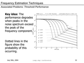
![Frequency Estimation Techniques Associated Problems: Threshold Performance [continued] For the multi-harmonic case, two threshold mechanisms occur: the noise outlier case and rational harmonic locking. This means that, sometimes, ½, 1/3, 2/3, 2 or 3 times the true frequency is estimated.](https://image.slidesharecdn.com/compdspKootsookosFrequencyEstimation-122758273435-phpapp01/85/Frequency-Estimation-33-320.jpg)


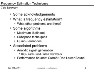
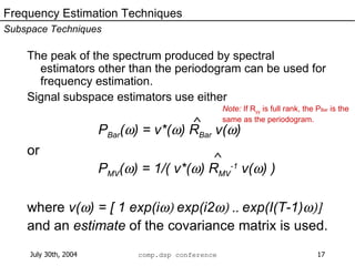
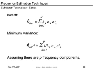
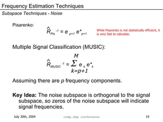
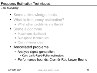
This document discusses various techniques for frequency estimation from signals. It summarizes maximum likelihood estimation, subspace techniques like MUSIC, the Quinn-Fernandes method, analytic signal generation to enable frequency estimation of real signals, and performance bounds like the Cramér-Rao lower bound. It also mentions Kay's estimator and related weighted frequency estimators that aim to minimize mean square error.