Downloaded 12 times
![(PAGE # 10) PREPARED BY: MUHAMMAD MEMON
SAMPLING DISTRIBUTION
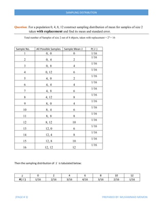
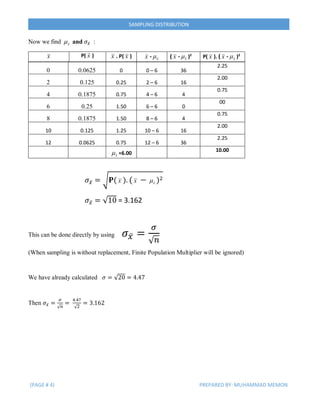
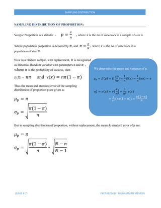
Question: A company employs 2000 persons, 600 of whom are post-graduates.
(i) Specify completely the sampling distribution of proportion of post-
graduates for samples of size 50 drawn without replacement.
(ii) Find the probability of selection a sample whose proportion of post-
graduates is greater than 0.4.
Solution:
(i) The population proportion of post-graduates is 𝜋 =
600
2000
= 0.3
Since 𝒏 ≥ 𝟓𝟎 & 𝒏𝝅 = 50 ∗ 0.3 = 15 ; 𝒏( 𝟏 − 𝝅) = 𝟓𝟎 ∗ 𝟎. 𝟕 = 𝟑𝟓
are both greater than 5, the sampling distribution of sample proportion may be
considered normal with parameters
𝜇 𝑝 = 𝜋 = 0.3 [Since
𝑛
𝑁
=
50
2000
< 0.05 therefore f.p.m will be ignored.]
𝜎 𝑝
2
=
𝜋(1−𝜋)
𝑛
=
0.3∗0.7
50
= 0.0042
(ii) Since the sampling distribution of p has been determined as normal, therefore z-
transformation is used to find probabilities.
𝒛 =
𝒑 − 𝝅
√ 𝝅(𝟏 − 𝝅)
𝒏
=
𝟎. 𝟒 − 𝟎. 𝟑
√𝟎. 𝟎𝟎𝟒𝟐
= 𝟏. 𝟓𝟒
P(𝒑 > 𝟎. 𝟒) = 𝑷(𝒛 > 𝟏. 𝟓𝟒)
= 0.5 − 𝑃(0 ≤ 𝑧 ≤ 1.54)
= 0.5 − 0.4382 = 0.0618](https://image.slidesharecdn.com/8cebe8ac-3f3f-4311-a621-edb945435b9e-160928071749/85/Sampling-Distribution-I-10-320.jpg)

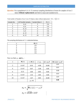
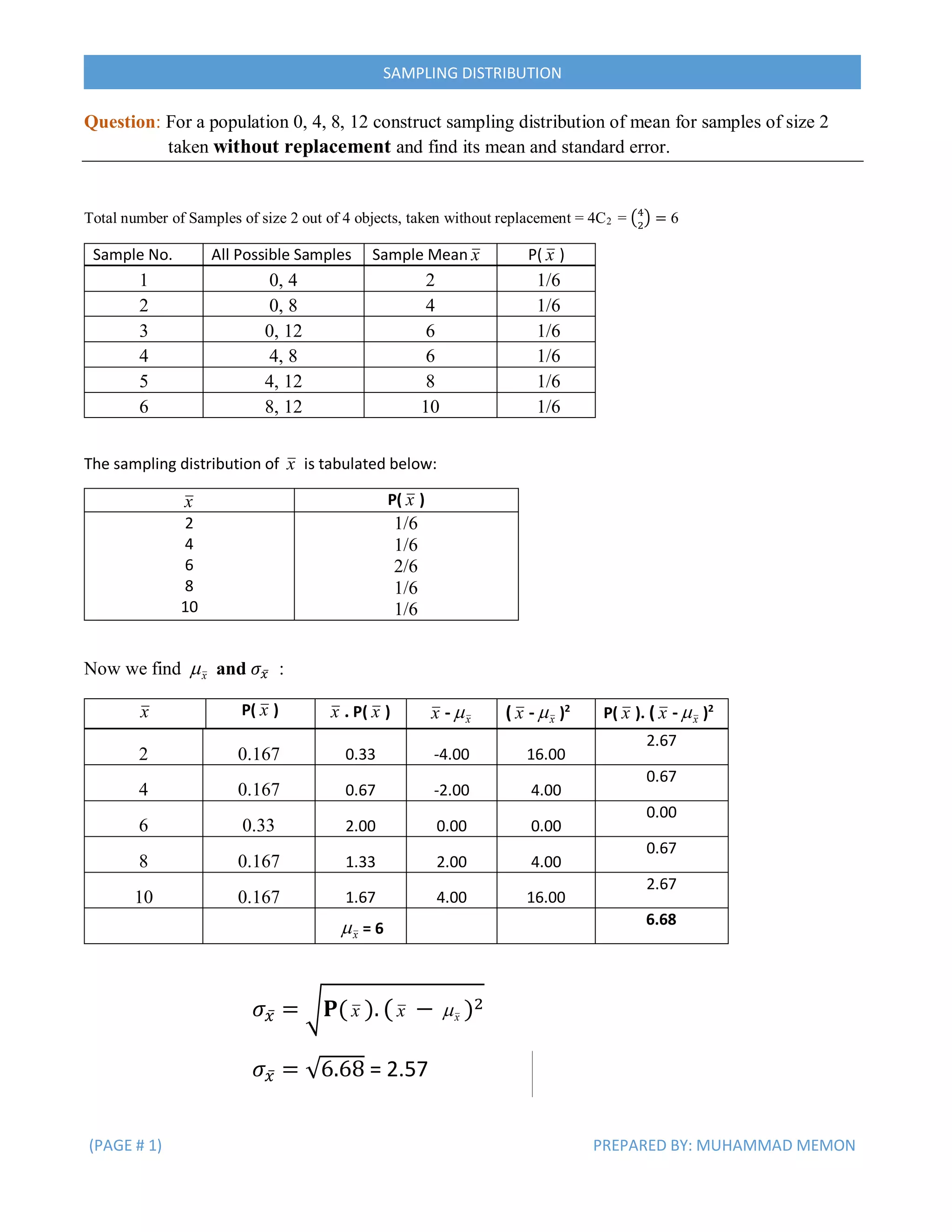
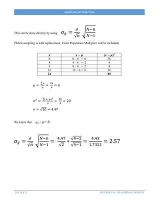
This document discusses sampling distributions and their properties. It contains examples of constructing sampling distributions of the mean for samples taken from populations with and without replacement. The mean and standard error of these sampling distributions are calculated. The central limit theorem is explained, noting that the sampling distribution of the mean approaches a normal distribution as sample size increases. Sampling distributions of proportions are also discussed, and formulas are provided for the mean and variance of such distributions. Examples are included to demonstrate these concepts.