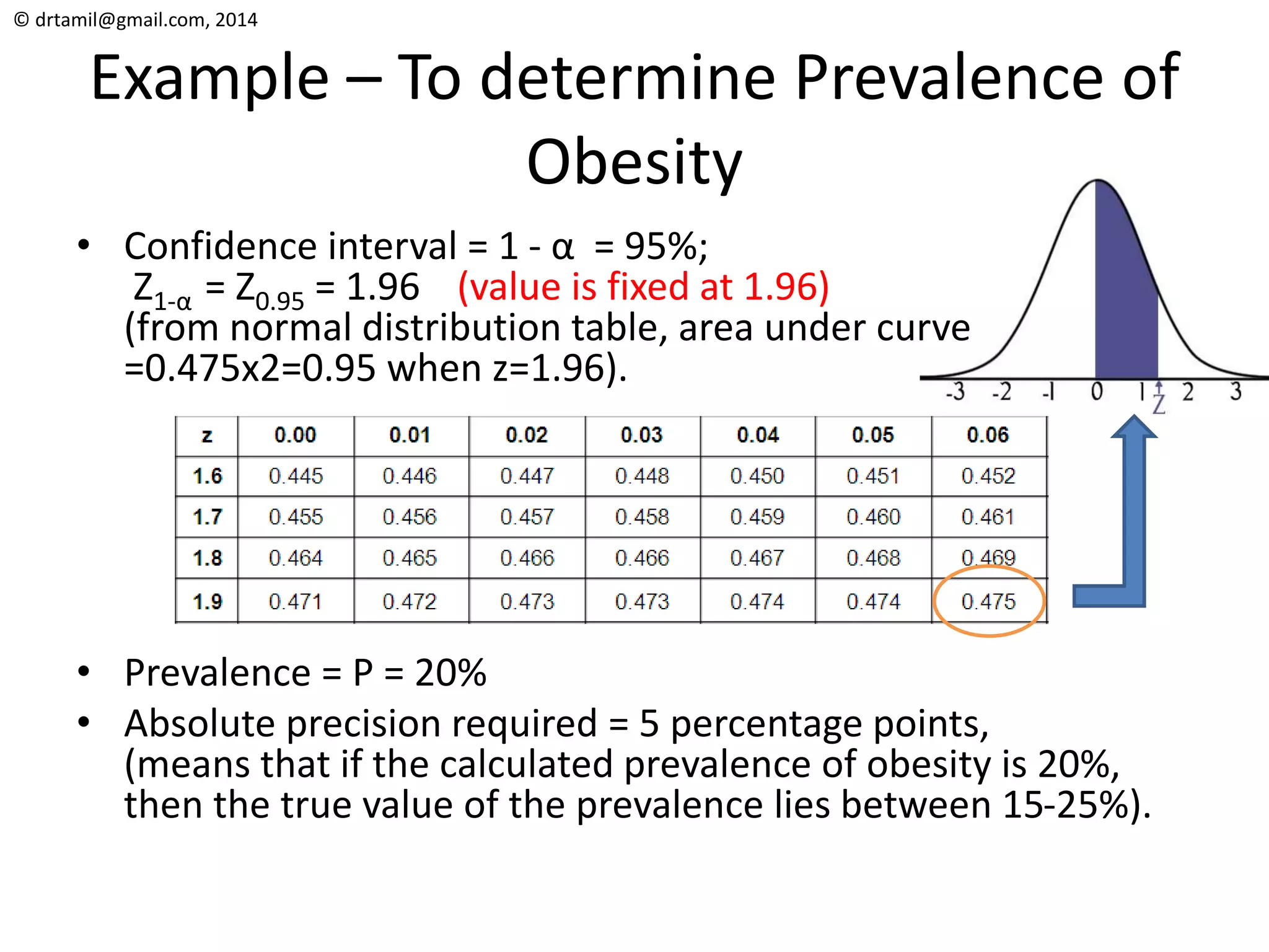
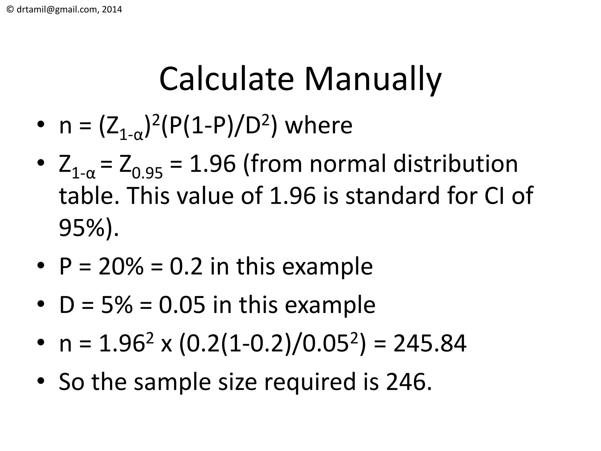
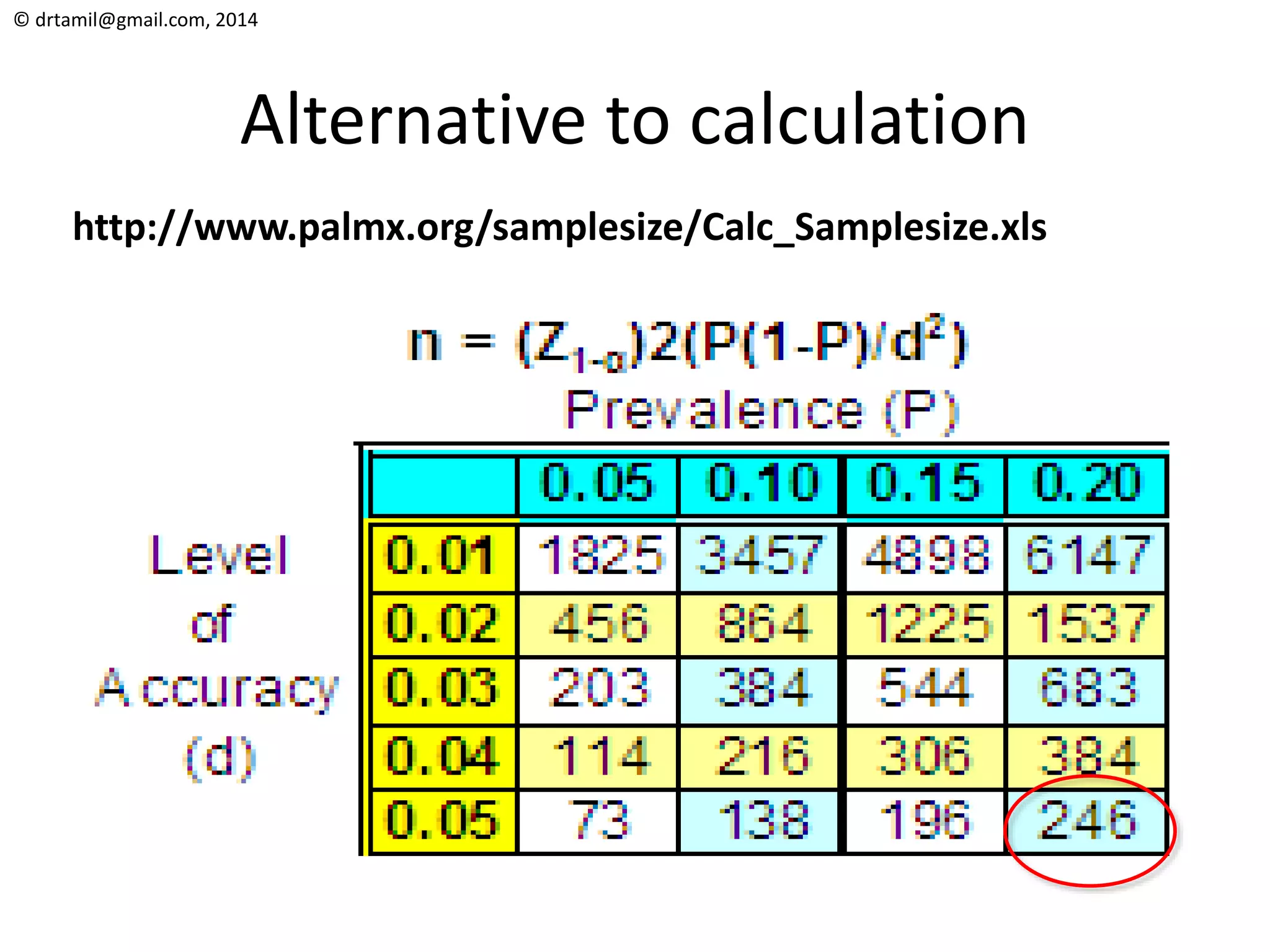
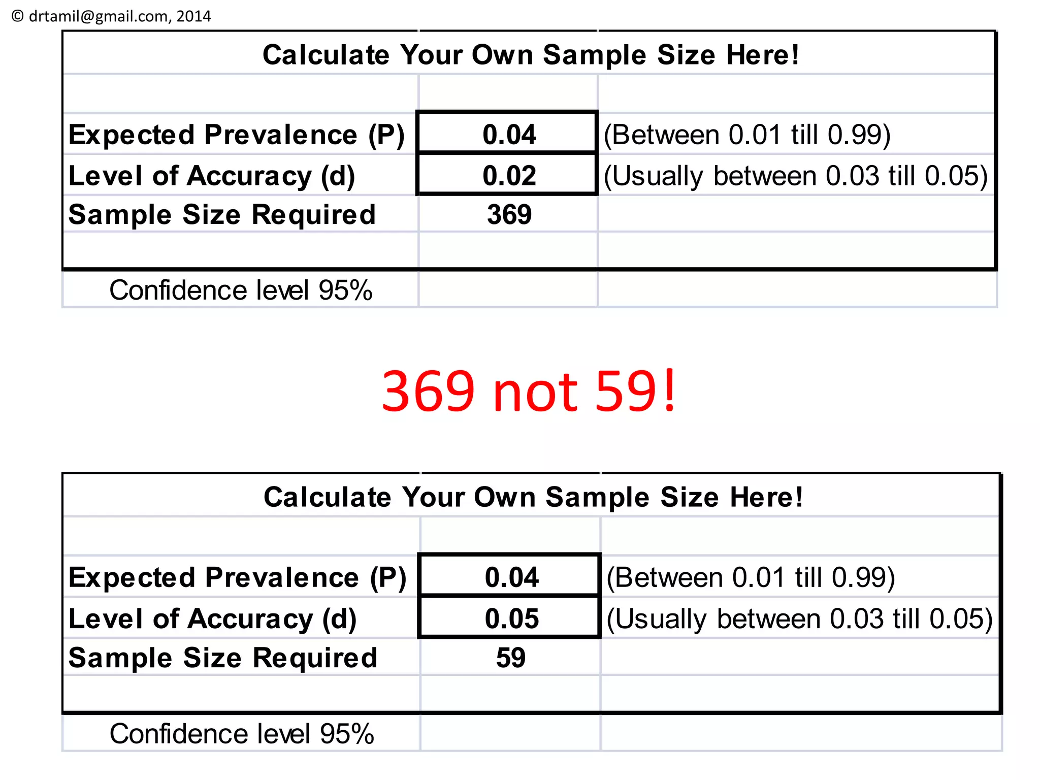
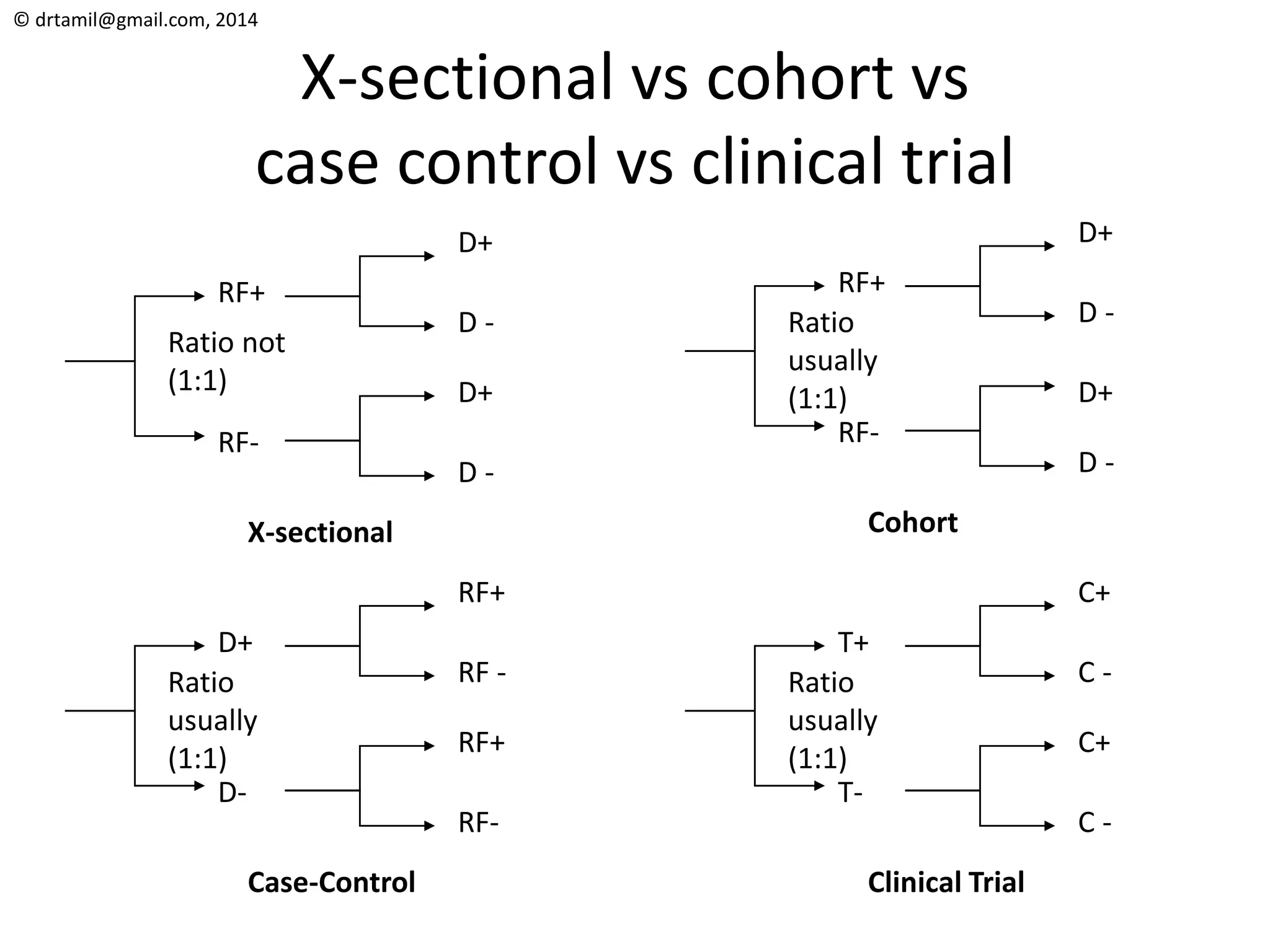
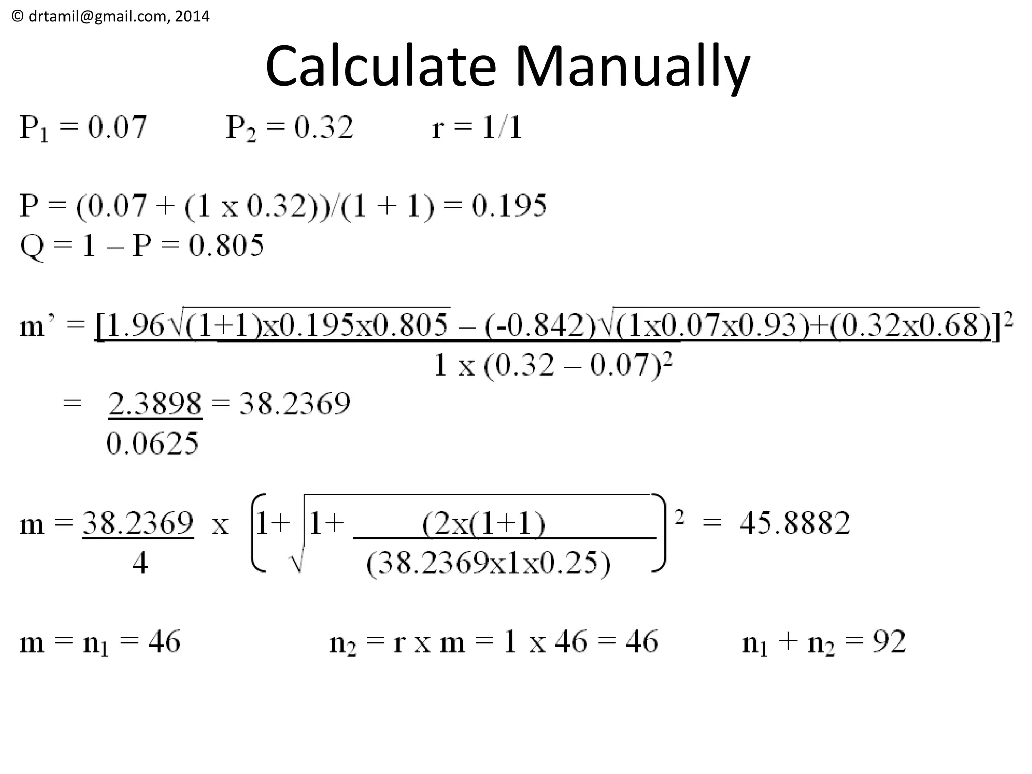
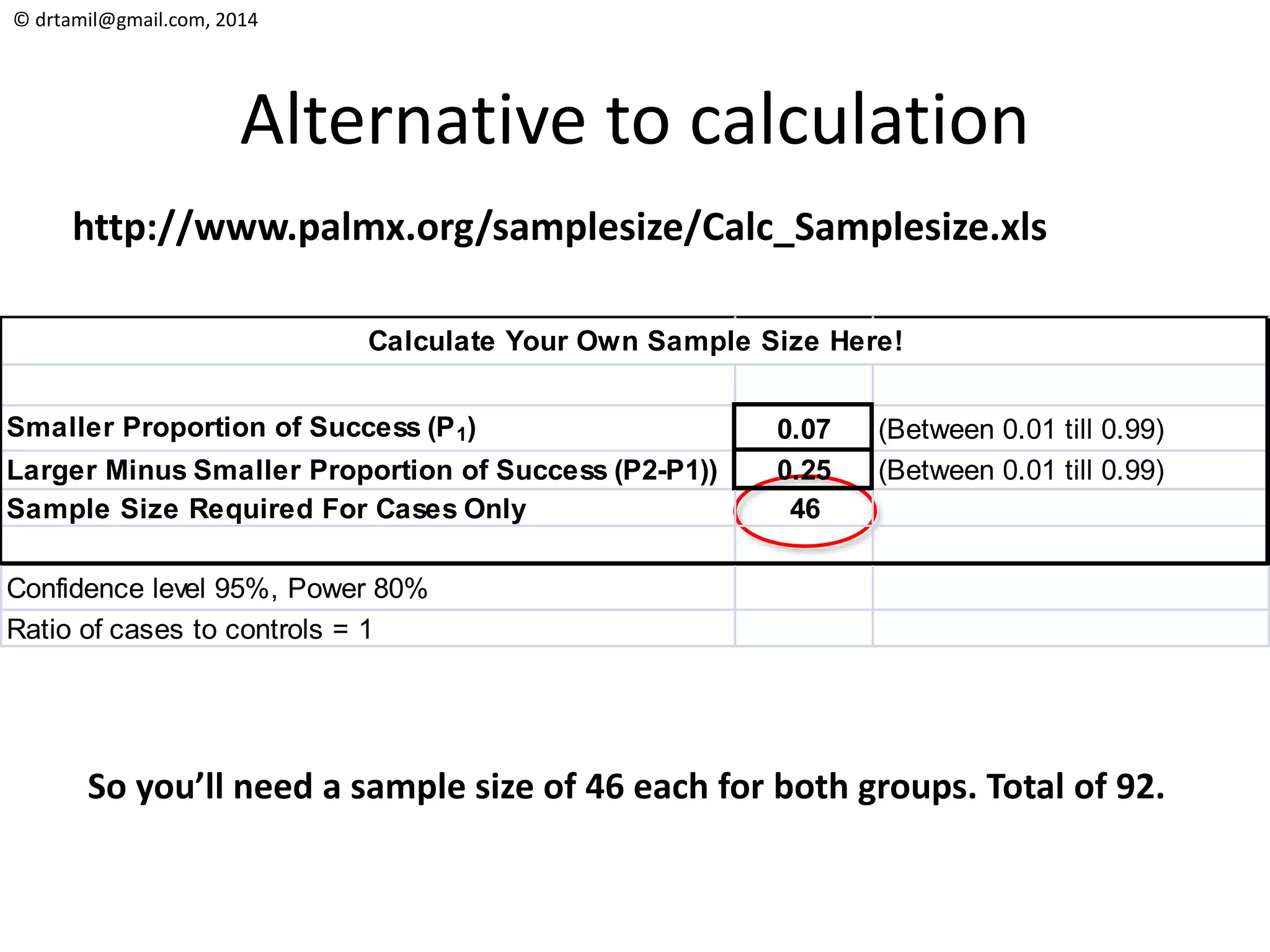
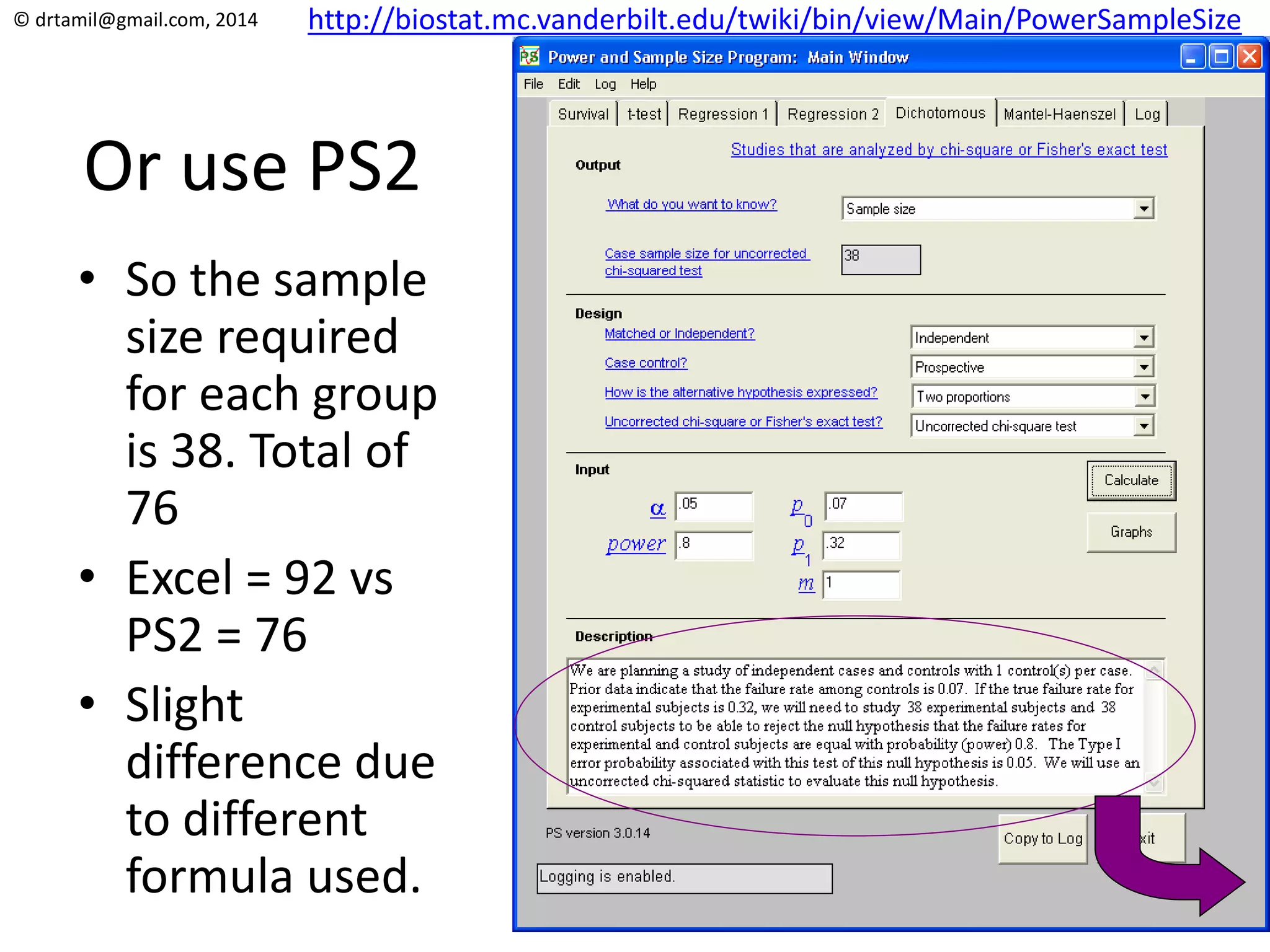
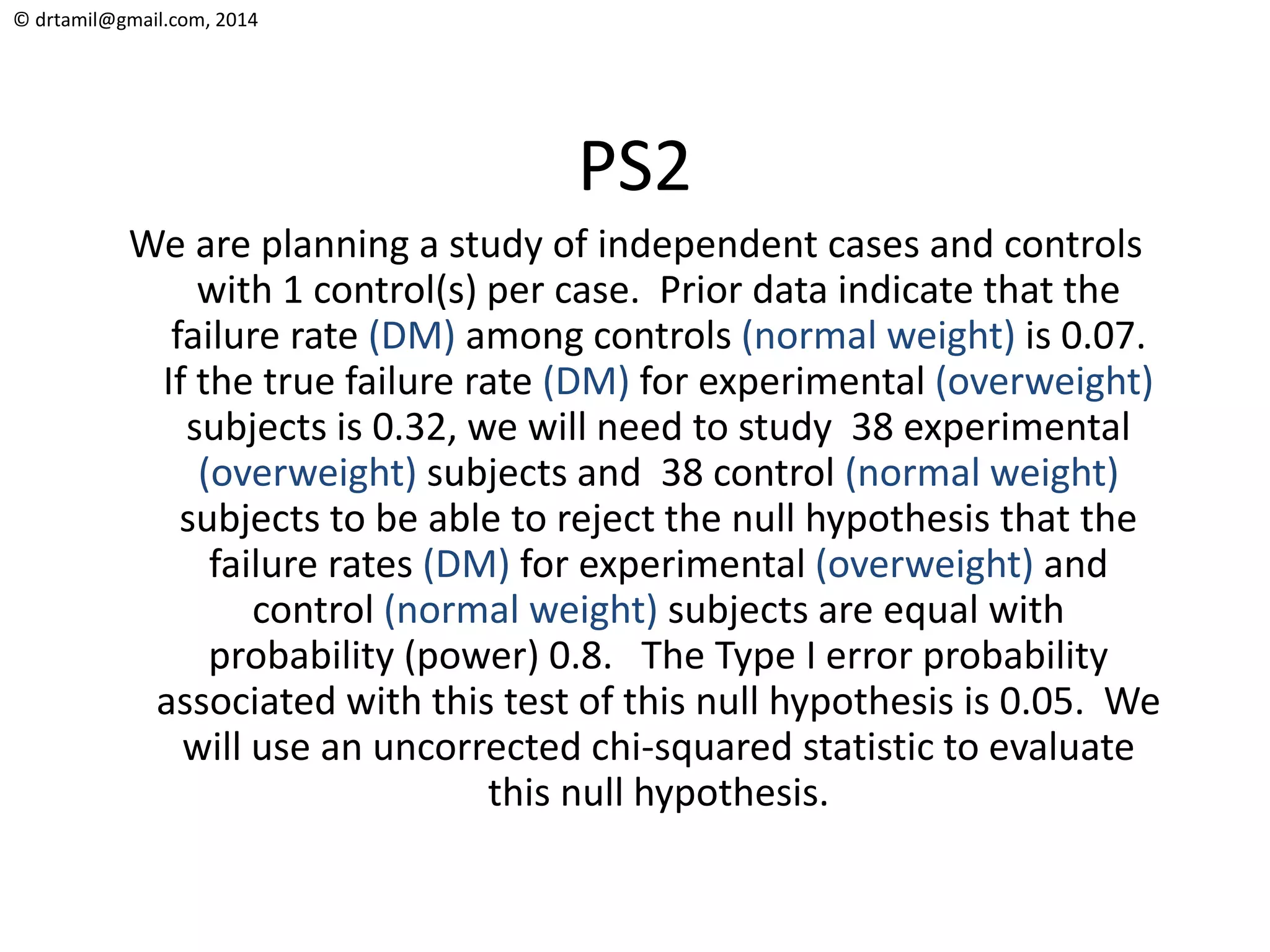
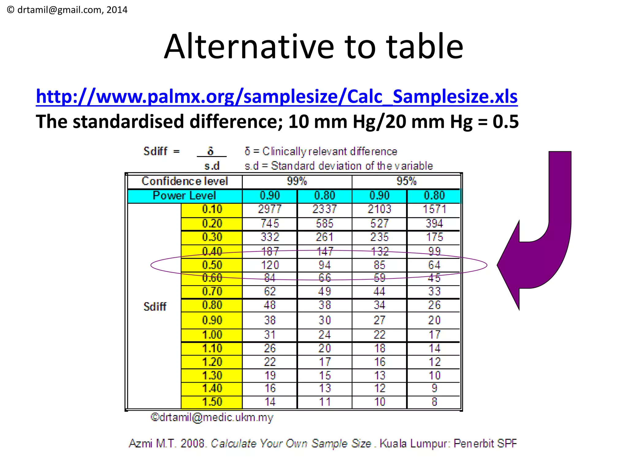
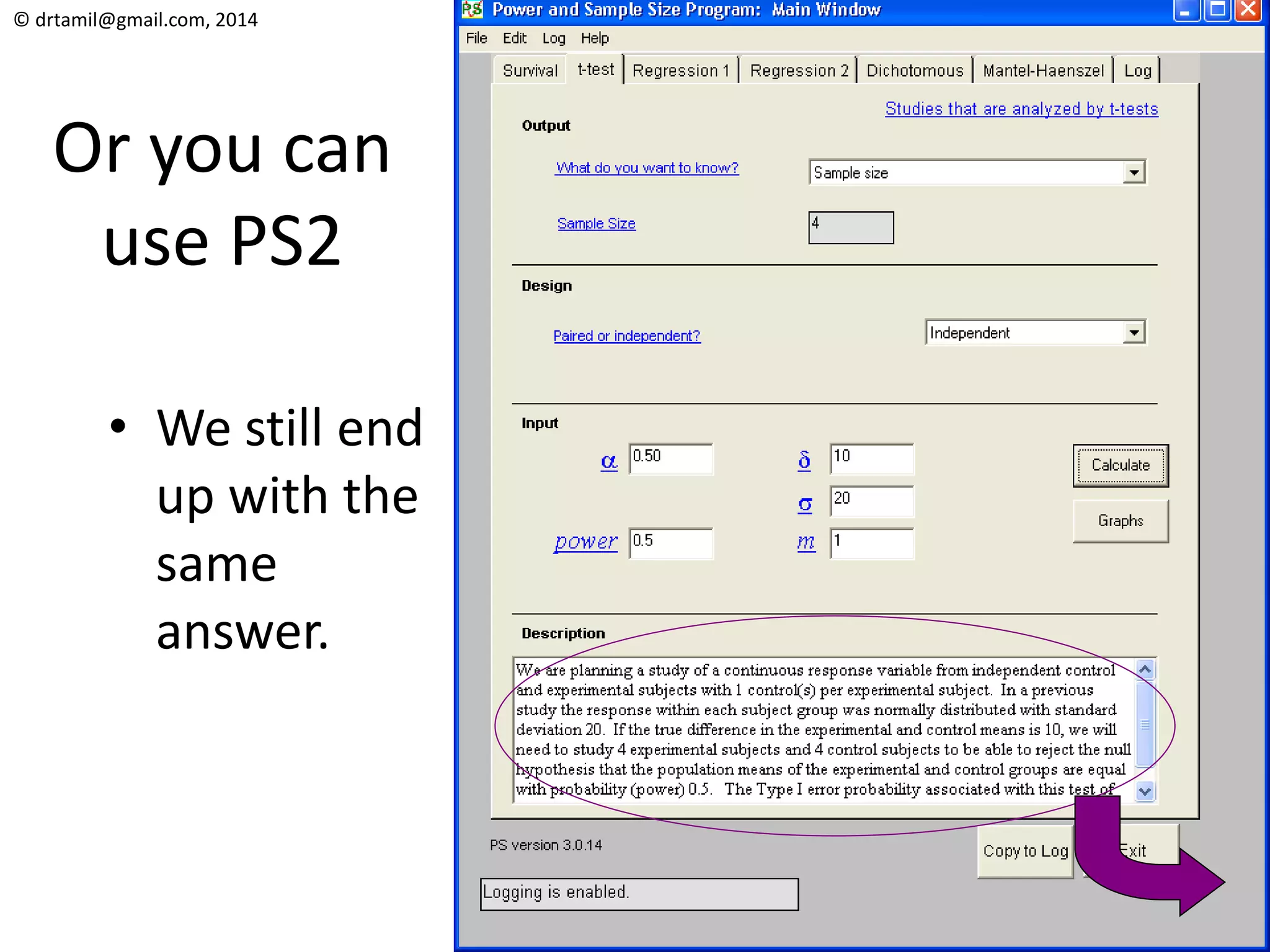
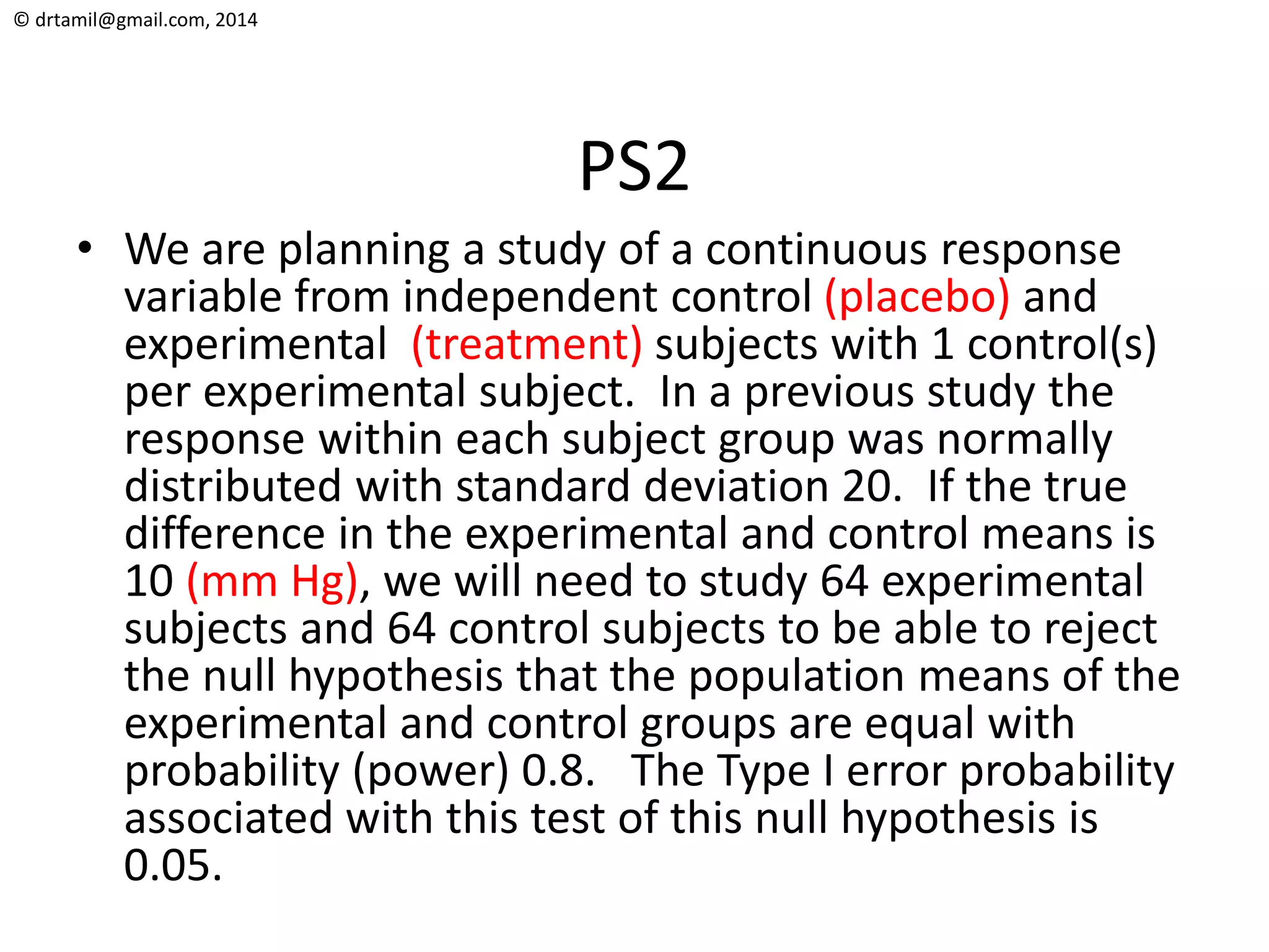
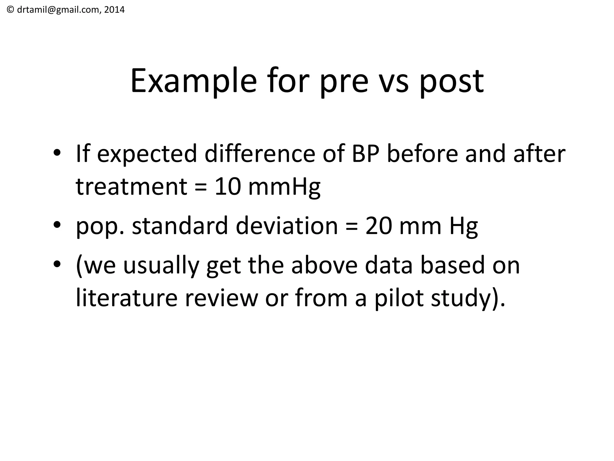
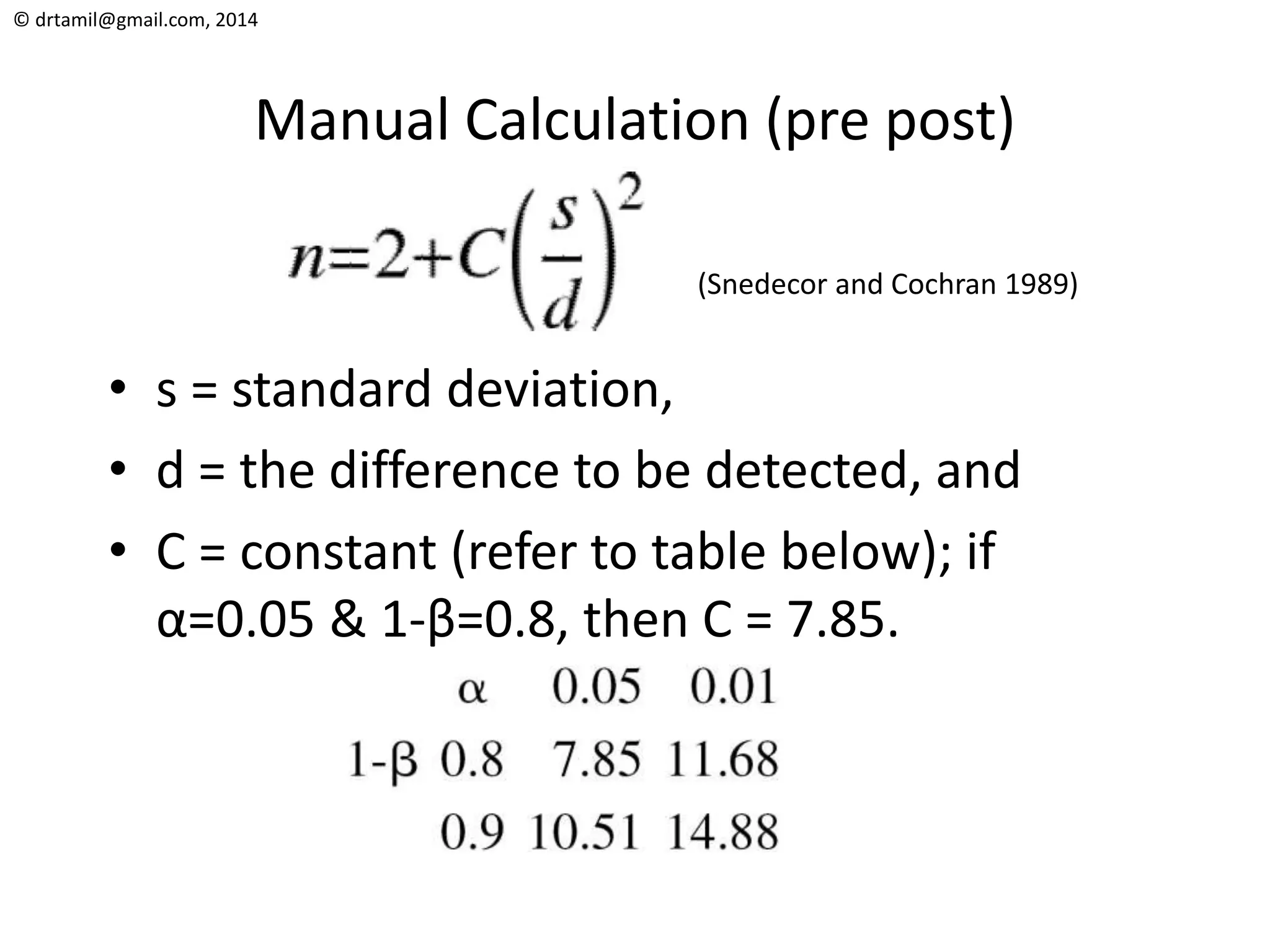
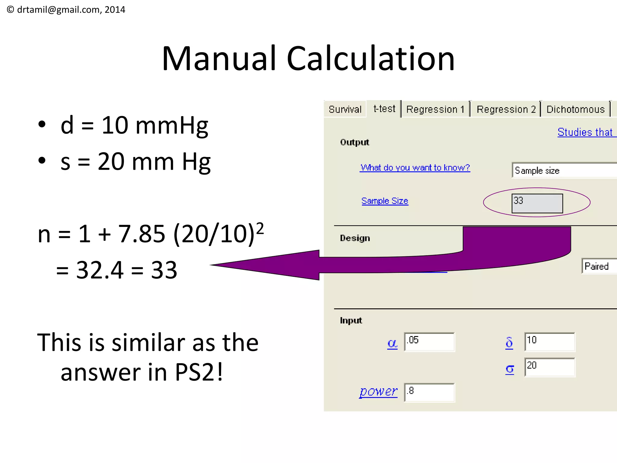
Sample size calculation - a brief overview

© drtamil@gmail.com, 2014
Sample size calculation
Research Week 2014
Health Cluster UKM

Introduction
• This is an abbreviated set of slides on how to
calculate sample size.
• It will focus on those with
– Measuring prevalence/incidence for outcome
– Qualitative outcome (i.e. Dead vs Alive)
– Continuous outcome (i.e. drop of BP in mm Hg)
for commonly used study designs in PPUKM.
• Those who want the complete set of slides for
calculating sample size, please refer to next page;

Sample Size Calculation on Slideshare
1. Why do we need to calculate sample size?
2. Tools to calculate sample size
3. Calculate sample size for prevalence studies
4. Calculate sample size for cross-sectional studies
5. Calculate sample size for case-control studies
6. Calculate sample size for cohort studies
7. Calculate sample size for clinical trials
8. Calculate sample size for clinical trials (continuous
outcome)
9. Calculate sample size for diagnostic study
10. eBook

Measuring prevalence
Calculate sample size

Prevalence
• If the objective of your study is to measure the
prevalence of the outcome of interest, then
you will be conducting a cross-sectional study.
So you will only take a sample of your
population. The number of sample selected
depends on the expected prevalence rate.
• To estimate the expected prevalence rate, you
will need to do a literature review, hopefully
similar to your own population.

Prevalence – Sample size
• Do a literature review to estimate the
prevalence for the outcome of interest
being studied.
• Determine the absolute precision
required i.e. 5% (usually between 3% to
5%).
• Calculate manually using (Kish L. 1965)
n = (Z1-α)2(P(1-P)/D2)
• Or use the attached Excel file.

Example – To determine Prevalence of
Obesity
• Confidence interval = 1 - α = 95%;
Z1-α = Z0.95 = 1.96 (value is fixed at 1.96)
(from normal distribution table, area under curve
=0.475x2=0.95 when z=1.96).
• Prevalence = P = 20%
• Absolute precision required = 5 percentage points,
(means that if the calculated prevalence of obesity is 20%,
then the true value of the prevalence lies between 15-25%).

Calculate Manually
• n = (Z1-α)2(P(1-P)/D2) where
• Z1-α = Z0.95 = 1.96 (from normal distribution
table. This value of 1.96 is standard for CI of
95%).
• P = 20% = 0.2 in this example
• D = 5% = 0.05 in this example
• n = 1.962 x (0.2(1-0.2)/0.052) = 245.84
• So the sample size required is 246.

Alternative to calculation
http://www.palmx.org/samplesize/Calc_Samplesize.xls

Reminder
• If the prevalence for the outcome of interest is
less than 5%, you should not be doing a cross-
sectional study, instead you should be doing a
case-control study.
• If your supervisor still insists that you do x-
sectional study, then the level of precision
should be half of the prevalence; i.e. prevalence
of HIV among STD patients is 4% therefore
accuracy (d) must be set at 2%. Therefore the
required sample size would be 369, not 59.

Expected Prevalence (P) 0.04 (Between 0.01 till 0.99)
Level of Accuracy (d) 0.02 (Usually between 0.03 till 0.05)
Sample Size Required 369
Confidence level 95%
Calculate Your Own Sample Size Here!
Expected Prevalence (P) 0.04 (Between 0.01 till 0.99)
Level of Accuracy (d) 0.05 (Usually between 0.03 till 0.05)
Sample Size Required 59
Confidence level 95%
369 not 59!

Dichotomous Qualitative
Outcome
Calculate sample size

X-sectional vs cohort vs
case control vs clinical trial
D+
RF+
RF-
D -
D+
D -
Ratio not
(1:1)
X-sectional
D+
D-
RF -
RF+
RF-
Ratio
usually
(1:1)
Case-Control
D -
RF+
RF-
D -
D+
Ratio
usually
(1:1)
Cohort
D+
RF+
T+
T-
C -
C+
C -
Ratio
usually
(1:1)
Clinical Trial
C+

Example – overweight have higher risk
of DM
From literature review, identify the rate of disease among
those with & without the risk factor.
• Ratio of unexposed (Normal) vs exposed (Overweight);
1:1
• Equal ratio therefore equal proportion of sample from
no-risk (Normal) and from at-risk (Overweight)
population.
• P1=true proportion of DM in no-risk (Normal) population
= 7%
• P2=true proportion of DM in at-risk (Overweight)
population =32%
• (Rifas-Shiman SL et al, 2008.Diabetes and lipid screening
among patients in primary care: A cohort study. BMC
Health Services Research.)

From Literature Review: Obesity &
Diabetes M.
Normal
Overweight
DM - (68%)
DM + (32%)
DM + (7%)
DM - (93%)
Sample
ratio (1:1)
Rifas-Shiman SL et al, 2008.Diabetes and lipid screening among patients in primary care: A cohort study. BMC Health Services Research.

Calculate Manually
Calculate using these formulas (Fleiss JL. 1981. pp. 44-45)
m=n1=size of sample from population 1 n2=size of sample from population 2
P1=proportion of disease in population 1 P2=proportion of disease in population 2
α= "Significance” = 0.05 β=chance of not detecting a difference = 0.2
1-β = Power = 0.8 r = n2/n1 = ratio of cases to controls
P = (P1+rP2)/(r+1) Q = 1-P.
n1 = m n2 = rm
From table A.2 in Fleiss;
• If 1- α is 0.95 then cα/2 is 1.960
• If 1- β is 0.80 then c1-beta is -0.842

Calculate Manually

Alternative to calculation
Smaller Proportion of Success (P1) 0.07 (Between 0.01 till 0.99)
Larger Minus Smaller Proportion of Success (P2-P1)) 0.25 (Between 0.01 till 0.99)
Sample Size Required For Cases Only 46
Confidence level 95%, Power 80%
Ratio of cases to controls = 1
So you’ll need a sample size of 46 each for both groups. Total of 92.

Or use PS2
• So the sample
size required
for each group
is 38. Total of
76
• Excel = 92 vs
PS2 = 76
• Slight
difference due
to different
formula used.
http://biostat.mc.vanderbilt.edu/twiki/bin/view/Main/PowerSampleSize

PS2
We are planning a study of independent cases and controls
with 1 control(s) per case. Prior data indicate that the
failure rate (DM) among controls (normal weight) is 0.07.
If the true failure rate (DM) for experimental (overweight)
subjects is 0.32, we will need to study 38 experimental
(overweight) subjects and 38 control (normal weight)
subjects to be able to reject the null hypothesis that the
failure rates (DM) for experimental (overweight) and
control (normal weight) subjects are equal with
probability (power) 0.8. The Type I error probability
associated with this test of this null hypothesis is 0.05. We
will use an uncorrected chi-squared statistic to evaluate
this null hypothesis.

Sample size calculation -
Outcome is continuous data
Jones SR, Carley S & Harrison M.
An introduction to power and sample size estimation.
Emergency Medical Journal 2003;20;453-458. 2003

Example (two groups)
• If expected difference of BP between two
treatment groups = 10 mmHg
• pop. standard deviation = 20 mm Hg
• (we usually get the above data based on
literature review or from a pilot study).

Manual Calculation (2 groups)
• s = standard deviation,
• d = the difference to be detected, and
• C = constant (refer to table below); if
α=0.05 & 1-β=0.8, then C = 7.85.
(Snedecor and Cochran 1989)

Manual Calculation
• d = 10 mmHg
• s = 20 mm Hg
n = 1 + 2 x 7.85 (20/10)2
= 63.8 = 64
We will need 64 samples per treatment group. For
two treatment groups, that will be a total of 128
samples.

Alternative to table
The standardised difference; 10 mm Hg/20 mm Hg = 0.5

Or you can
use PS2
• We still end
up with the
same
answer.

PS2
• We are planning a study of a continuous response
variable from independent control (placebo) and
experimental (treatment) subjects with 1 control(s)
per experimental subject. In a previous study the
response within each subject group was normally
distributed with standard deviation 20. If the true
difference in the experimental and control means is
10 (mm Hg), we will need to study 64 experimental
subjects and 64 control subjects to be able to reject
the null hypothesis that the population means of the
experimental and control groups are equal with
probability (power) 0.8. The Type I error probability
associated with this test of this null hypothesis is
0.05.

Example for pre vs post
• If expected difference of BP before and after
treatment = 10 mmHg
• pop. standard deviation = 20 mm Hg
• (we usually get the above data based on
literature review or from a pilot study).

Manual Calculation (pre post)
• s = standard deviation,
• d = the difference to be detected, and
• C = constant (refer to table below); if
α=0.05 & 1-β=0.8, then C = 7.85.
(Snedecor and Cochran 1989)

Manual Calculation
• d = 10 mmHg
• s = 20 mm Hg
n = 1 + 7.85 (20/10)2
= 32.4 = 33
This is similar as the
answer in PS2!

Next
Exploring your data

Sample size calculation - a brief overview

More Related Content

What's hot

Viewers also liked

Similar to Sample size calculation - a brief overview

More from Azmi Mohd Tamil

Recently uploaded

In this document

Sample size calculation - a brief overview