Few topics of statistics and probability for beginners with source link

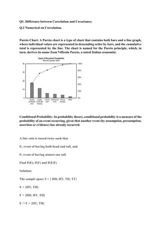
1. Q1. Difference between Correlation and Covariance.
Q.2 Numerical on Correlation.
Pareto Chart: A Pareto chart is a type of chart that contains both bars and a line graph,
where individual values are represented in descending order by bars, and the cumulative
total is represented by the line. The chart is named for the Pareto principle, which, in
turn, derives its name from Vilfredo Pareto, a noted Italian economist.
Conditional Probability: In probability theory, conditional probability is a measure of the
probability of an event occurring, given that another event (by assumption, presumption,
assertion or evidence) has already occurred.
A fair coin is tossed twice such that
E: event of having both head and tail, and
F: event of having atmost one tail.
Find P(E), P(F) and P(E|F)
Solution:
The sample space S = { HH, HT, TH, TT}
E = {HT, TH}
F = {HH, HT, TH}
E ∩ F = {HT, TH}

2. P(E) = 2/4 = ½
P(F) = ¾
P(E ∩ F) = 2/4 = ½
P(E|F) = P(E ∩ F)/P(F) = ½ ÷ ¾ = ⅔.
What is the difference between conditional probability and Bayes Theorem ?
The given questions belong to the concepts of probability. To state out the differences
between Bayes Theorem and Conditional Probability, first we must have an idea of their
origin. So, Bayes Theorem is a formula that describes how to update the probabilities of
hypotheses when given evidence. It follows simply from the axioms of conditional
probability, but can be used to powerfully reason about a wide range of problems. And,
conditional probability is the probability of one thing given that another thing is true.
Also, Conditional Probability is the base concept in Bayes Theorem.
What is the difference between conditional probability and Bayes Theorem ?
(vedantu.com)
What is the difference between Bayes theorem and naive Bayes?
Well, you need to know that the distinction between Bayes theorem and Naive Bayes is
that Naive Bayes assumes conditional independence where Bayes theorem does not. This
means the relationship between all input features are independent. Maybe not a great
assumption, but this is why the algorithm is called “naive”.
What is binomial distribution?
https://www.intellspot.com/binomial-distribution-examples/
In simple words, a binomial distribution is the probability of a success or failure results
in an experiment that is repeated a few or many times.
The prefix “bi” means two. We have only 2 possible incomes.
Binomial probability distributions are very useful in a wide range of problems,
experiments, and surveys. However, how to know when to use them?
Let’s see the necessary conditions and criteria to use binomial distributions:
Rule 1: Situation where there are only two possible mutually exclusive outcomes (for
example, yes/no survey questions).
Rule2: A fixed number of repeated experiments and trials are conducted (the process
must have a clearly defined number of trials).

3. Rule 3: All trials are identical and independent (identical means every trial must be
performed the same way as the others; independent means that the result of one trial does
not affect the results of the other subsequent trials).
Rule 4: The probability of success is the same in every one of the trials.
Notations for Binomial Distribution and the Mass Formula:
Where:
p is the probability of success on any trail.
q = 1- p – the probability of failure
n – the number of trails/experiments
x – the number of successes, it can take the values 0, 1, 2, 3, . . . n.
nCx = n!/x!(n-x) and denotes the number of combinations of n elements taken x at a time.
Assuming what the nCx means, we can write the above formula in this way:
Just to remind that the ! symbol after a number means it’s a factorial. The factorial of a
non-negative integer x is denoted by x!. And x! is the product of all positive integers less
than or equal to x. For example, 4! = 4 x 3 x 2 x 1 = 24.
Examples of binomial distribution problems:
The number of defective/non-defective products in a production run.
Yes/No Survey (such as asking 150 people if they watch ABC news).
Vote counts for a candidate in an election.
The number of successful sales calls.
The number of male/female workers in a company
So, as we have the basis let’s see some binominal distribution examples, problems, and
solutions from real life.
Example 1:

4. Let’s say that 80% of all business startups in the IT industry report that they generate a
profit in their first year. If a sample of 10 new IT business startups is selected, find the
probability that exactly seven will generate a profit in their first year.
First, do we satisfy the conditions of the binomial distribution model?
There are only two possible mutually exclusive outcomes – to generate a profit in the first
year or not (yes or no).
There are a fixed number of trails (startups) – 10.
The IT startups are independent and it is reasonable to assume that this is true.
The probability of success for each startup is 0.8.
We know that:
n = 10, p=0.80, q=0.20, x=7
The probability of 7 IT startups to generate a profit in their first year is:
This is equivalent to:
Interpretation/solution: There is a 20.13% probability that exactly 7 of 10 IT startups will
generate a profit in their first year when the probability of profit in the first year for each
startup is 80%.
And as we live in the internet ERA and there are so many online calculators available for
free use, there is no need to calculate by hand.
What is Normal Distribution?
Normal Distribution (mathsisfun.com)
The normal distribution is a continuous probability distribution function also known as
Gaussian distribution which is symmetric about its mean and has a bell-shaped curve. It
is one of the most used probability distributions. Two parameters characterize it
Mean(μ)- It represents the center of the distribution
Standard Deviation(σ) – It represents the spread in the curve
The formula for Normal distribution is

5. Properties Of Normal Distribution
Symmetric distribution – The normal distribution is symmetric about its mean point. It
means the distribution is perfectly balanced toward its mean point with half of the data
on either side.
Bell-Shaped curve – The graph of a normal distribution takes the form bell-shaped curve
with most of the points accumulated at its mean position. The shape of this curve is
determined by the mean and standard deviation of the distribution
Empirical Rule – The normal distribution curve follows the empirical rule where 68% of
the data lies within 1 standard deviation from the mean of the graph, 95% of the data lies
within 2 standard deviations from the mean and 97% of the data lies within 3 standard
deviations from the mean.
Additive Rule – The sum of two or more normal distributions will always be a normal
distribution.
Central Limit Theorem – It states if we take the mean of large no data points collected
from independent and identical distributed random variables then this mean will follow
a normal distribution regardless of their original distribution.
Let’s understand the daily life examples of Normal Distribution.
1. Height: The height of people is an example of normal distribution. Most of the
people in a specific population are of average height. The number of people taller

6. and shorter than the average height people is almost equal, and a very small
number of people are either extremely tall or extremely short. Several genetic and
environmental factors influence height. Therefore, it follows the normal
distribution.
2. Rolling A Dice: A fair rolling of dice is also a good example of normal distribution.
In an experiment, it has been found that when a dice is rolled 100 times, chances
to get ‘1’ are 15-18% and if we roll the dice 1000 times, the chances to get ‘1’ is,
again, the same, which averages to 16.7% (1/6). If we roll two dice simultaneously,
there are 36 possible combinations. The probability of rolling ‘1’ (with six possible
combinations) again averages to around 16.7%, i.e., (6/36). More the number of
dice more elaborate will be the normal distribution graph.
Other Examples are:
IQ, Blood Pressure, Shoe Size, Birth Weight, Student’s Average Report.

7. Range: It is the given measure of how spread apart the values in a
data set are.
Range = Highest Value – Lowest Value
Or
Range = Highest observation – Lowest observation
Or
Range = Maximum value – Minimum Value
Solved Examples
Example 1: Find the range of given observations: 32, 41, 28, 54, 35, 26, 23, 33, 38, 40.
Solution: Let us first arrange the given values in ascending order.
23, 26, 28, 32, 33, 35, 38, 40, 41, 54
Since 23 is the lowest value and 54 is the highest value, therefore, the range of the
observations will be;
Range (X) = Max (X) – Min (X)
= 54 – 23
= 31
Hence, 31 is the required answer.
Example 2: Following are the marks of students in Mathematics: 50, 53, 50, 51, 48, 93,
90, 92, 91, 90. Find the range of the marks.

8. Solution: Arrange the following marks in ascending order, we get;
48, 50, 50, 51, 53, 90, 90, 91, 92, 93
Thus, the range of marks will be:
Range = Maximum marks – Minimum marks
Range = 93 – 48 = 45
Thus, 45 is the required range.
Inter Quartile Range (IQR): It is the measure of variability, based on dividing a data set
into quartiles. https://www.scribbr.com/statistics/interquartile-range/
The interquartile range (IQR) contains the second and third quartiles, or the middle half
of your data set. Whereas the range gives you the spread of the whole data set, the
interquartile range gives you the range of the middle half of a data set.
Calculate the interquartile range by hand: The interquartile range is found by
subtracting the Q1 value from the Q3 value:
Formula Explanation
 IQR = interquartile range
 Q3 = 3rd quartile or 75th percentile
 Q1 = 1st quartile or 25th percentile
Q1 is the value below which 25 percent of the distribution lies, while Q3 is the value below
which 75 percent of the distribution lies.
You can think of Q1 as the median of the first half and Q3 as the median of the second
half of the distribution.

9. Methods for finding the interquartile range
Although there’s only one formula, there are various different methods for identifying
the quartiles. You’ll get a different value for the interquartile range depending on the
method you use.
Here, we’ll discuss two of the most commonly used methods. These methods differ
based on how they use the median.
Exclusive method vs inclusive method
The exclusive method excludes the median when identifying Q1 and Q3, while
the inclusive method includes the median in identifying the quartiles.
The procedure for finding the median is different depending on whether your data set is
odd- or even-numbered.
 When you have an odd number of data points, the median is the value in the
middle of your data set. You can choose between the inclusive and exclusive
method.
 With an even number of data points, there are two values in the middle, so the
median is their mean. It’s more common to use the exclusive method in this case.
While there is little consensus on the best method for finding the interquartile range, the
exclusive interquartile range is always larger than the inclusive interquartile range.
The exclusive interquartile range may be more appropriate for large samples, while for
small samples, the inclusive interquartile range may be more representative because it’s
a narrower range.
Steps for the exclusive method
To see how the exclusive method works by hand, we’ll use two examples: one with an
even number of data points, and one with an odd number.
Even-numbered data set
We’ll walk through four steps using a sample data set with 10 values.
Step 1: Order your values from low to high.
Step 2: Locate the median, and then separate the values below it from the values above it.

10. With an even-numbered data set, the median is the mean of the two values in the middle, so you
simply divide your data set into two halves.
Step 3: Find Q1 and Q3.
Q1 is the median of the first half and Q3 is the median of the second half. Since each of these halves
have an odd number of values, there is only one value in the middle of each half.
Step 4: Calculate the interquartile range.
Odd-numbered data set
This time we’ll use a data set with 11 values.
Step 1: Order your values from low to high.
Step 2: Locate the median, and then separate the values below it from the values above it.

11. In an odd-numbered data set, the median is the number in the middle of the list. The median itself is
excluded from both halves: one half contains all values below the median, and the other contains all
the values above it.
Step 3: Find Q1 and Q3.
Q1 is the median of the first half and Q3 is the median of the second half. Since each of these halves
have an odd-numbered size, there is only one value in the middle of each half.
Step 4: Calculate the interquartile range.
Steps for the inclusive method
Almost all of the steps for the inclusive and exclusive method are identical.
The difference is in how the data set is separated into two halves.
The inclusive method is sometimes preferred for odd-numbered data sets
because it doesn’t ignore the median, a real value in this type of data set.
Step 1: Order your values from low to high.

12. Step 2: Find the median.
The median is the number in the middle of the data set.
Step 2: Separate the list into two halves, and include the median in both halves.
The median is included as the highest value in the first half and the lowest value in the second half.
Step 3: Find Q1 and Q3.
Q1 is the median of the first half and Q3 is the median of the second half. Since the two halves each
contain an even number of values, Q1 and Q3 are calculated as the means of the middle values.
Step 4: Calculate the interquartile range.
We can see from these examples that using the inclusive method gives us a
smaller IQR. With the same data set, the exclusive IQR is 24, and the inclusive
IQR is 20.
When is the interquartile range useful?
The interquartile range is an especially useful measure of variability for
skewed distributions.

13. For these frequency distributions, the median is the best measure of central
tendency because it’s the value exactly in the middle when all values are
ordered from low to high.
Along with the median, the IQR can give you an overview of where most of
your values lie and how clustered they are.
The IQR is also useful for datasets with outliers. Because it’s based on the
middle half of the distribution, it’s less influenced by extreme values.
Visualize the interquartile range in boxplots
A boxplot, or a box-and-whisker plot, summarizes a data set visually using a
five-number summary.
Every distribution can be organized using these five numbers:
 Lowest value
 Q1: 25th percentile
 Median
 Q3: 75th percentile
 Highest value (Q4)
The vertical lines in the box show Q1, the median, and Q3, while the whiskers
at the ends show the highest and lowest values.

14. In a boxplot, the width of the box shows you the interquartile range. A smaller
width means you have less dispersion, while a larger width means you have
more dispersion.
An inclusive interquartile range will have a smaller width than an exclusive
interquartile range.
Boxplots are especially useful for showing the central tendency and
dispersion of skewed distributions.
The placement of the box tells you the direction of the skew. A box that’s
much closer to the right side means you have a negatively skewed
distribution, and a box closer to the left side tells you that you have a
positively skewed distribution.

15. Variance vs. standard deviation:
https://www.scribbr.com/statistics/variance/
The standard deviation is derived from variance and tells you, on average, how
far each value lies from the mean. It’s the square root of variance.
Both measures reflect variability in a distribution, but their units differ:
 Standard deviation is expressed in the same units as the original values (e.g.,
meters).
 Variance is expressed in much larger units (e.g., meters squared)
Since the units of variance are much larger than those of a typical value of a
data set, it’s harder to interpret the variance number intuitively. That’s why
standard deviation is often preferred as a main measure of variability.
However, the variance is more informative about variability than the standard
deviation, and it’s used in making statistical inferences.
Population vs. sample variance
Different formulas are used for calculating variance depending on whether you
have data from a whole population or a sample.
Population variance
When you have collected data from every member of the population that
you’re interested in, you can get an exact value for population variance.
The population variance formula looks like this:

16. Formula Explanation
 = population variance
 = sum of…
 Χ = each value
 = population mean
 Ν = number of values in the population
Sample variance
When you collect data from a sample, the sample variance is used to make
estimates or inferences about the population variance.
The sample variance formula looks like this:
Formula Explanation
 = sample variance
 = sum of…
 Χ = each value
 = sample mean
 n = number of values in the sample
With samples, we use n – 1 in the formula because using n would give us a
biased estimate that consistently underestimates variability. The sample
variance would tend to be lower than the real variance of the population.
Reducing the sample n to n – 1 makes the variance artificially large, giving you
an unbiased estimate of variability: it is better to overestimate rather than
underestimate variability in samples.
It’s important to note that doing the same thing with the standard deviation
formulas doesn’t lead to completely unbiased estimates. Since a square root
isn’t a linear operation, like addition or subtraction, the unbiasedness of the
sample variance formula doesn’t carry over the sample standard deviation
formula.
Steps for calculating the variance by hand
The variance is usually calculated automatically by whichever software you
use for your statistical analysis. But you can also calculate it by hand to better
understand how the formula works.
There are five main steps for finding the variance by hand. We’ll use a small
data set of 6 scores to walk through the steps.

17. Data set
466932605241
Step 1: Find the mean
To find the mean, add up all the scores, then divide them by the number of
scores.
Mean ( )
= (46 + 69 + 32 + 60 + 52 + 41) 6 = 50
Step 2: Find each score’s deviation from the mean
Subtract the mean from each score to get the deviations from the mean.
Since x
̅ = 50, take away 50 from each score.
ScoreDeviation from the mean
46 46 – 50 = -4
69 69 – 50 = 19
32 32 – 50 = -18
60 60 – 50 = 10
52 52 – 50 = 2
41 41 – 50 = -9
Step 3: Square each deviation from the mean
Multiply each deviation from the mean by itself. This will result in positive
numbers.

18. Squared deviations from the mean
(-4)2 = 4 × 4 = 16
192 = 19 × 19 = 361
(-18)2 = -18 × -18 = 324
102 = 10 × 10 = 100
22 = 2 × 2 = 4
(-9)2 = -9 × -9 = 81
Step 4: Find the sum of squares
Add up all of the squared deviations. This is called the sum of squares.
Sum of squares
16 + 361 + 324 + 100 + 4 + 81 = 886
Step 5: Divide the sum of squares by n – 1 or N
Divide the sum of the squares by n – 1 (for a sample) or N (for a population).
Since we’re working with a sample, we’ll use n – 1, where n = 6.
Variance
886 (6 – 1) = 886 5 = 177.2
Why does variance matter?
Variance matters for two main reasons:
 Parametric statistical tests are sensitive to variance.
 Comparing the variance of samples helps you assess group differences.

19. Homogeneity of variance in statistical tests
Variance is important to consider before performing parametric tests. These
tests require equal or similar variances, also called homogeneity of variance or
homoscedasticity, when comparing different samples.
Uneven variances between samples result in biased and skewed test results. If
you have uneven variances across samples, non-parametric tests are more
appropriate.
Using variance to assess group differences
Statistical tests like variance tests or the analysis of variance (ANOVA) use
sample variance to assess group differences. They use the variances of the
samples to assess whether the populations they come from differ from each
other.
Research example As an education researcher, you want to test the hypothesis that different
frequencies of quizzes lead to different final scores of college students. You collect the final scores
from three groups with 20 students each that had quizzes frequently, infrequently, or rarely over a
semester.
 Sample A: Once a week
 Sample B: Once every 3 weeks
 Sample C: Once every 6 weeks
To assess group differences, you perform an ANOVA.
The main idea behind an ANOVA is to compare the variances between groups
and variances within groups to see whether the results are best explained by
the group differences or by individual differences.
If there’s higher between-group variance relative to within-group variance,
then the groups are likely to be different as a result of your treatment. If not,
then the results may come from individual differences of sample members
instead.
Research exampleYour ANOVA assesses whether the differences in mean final scores between
groups come from the differences in the frequency of quizzes or the individual differences of the
students in each group.
To do so, you get a ratio of the between-group variance of final scores and the within-
group variance of final scores – this is the F-statistic. With a large F-statistic, you find
the corresponding p-value, and conclude that the groups are significantly different from
each other.