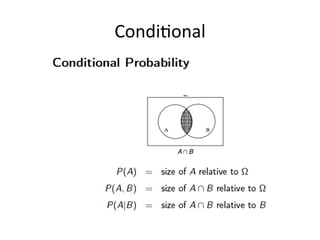
Download as PDF, PPTX
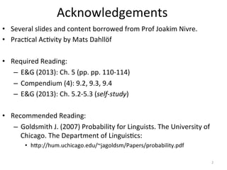

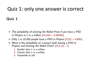
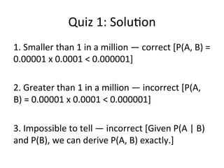
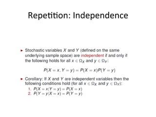
![Quiz
1:
Solu*on
1.
Smaller
than
1
in
a
million
—
correct
[P(A,
B)
=
0.00001(=100
000)
0.000001(=1
million)x
0.0001
(=10
000)
<
0.000001;
P
is
1
in
10
million]
2.
Greater
than
1
in
a
million
—
incorrect
[P(A,
B)
=
0.00001(=100
000)
0.000001(=1
million)x
0.0001
(=10
000)
<
0.000001;
P
is
1
in
10
million]
3.
Impossible
to
tell
—
incorrect
[Given
P(A
|
B)
and
P(B),
we
can
derive
P(A,
B)
exactly.]
10](https://image.slidesharecdn.com/42jointmarginalconditionalprobmath4lt-150316083455-conversion-gate01/85/Lecture-Joint-Conditional-and-Marginal-Probabilities-10-320.jpg)
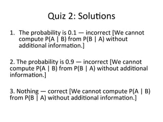
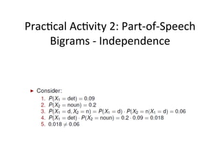
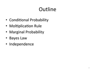
![Quiz
2:
Solu*ons
(Joakim’s
original)
1. The
probability
is
0.1
—
incorrect
[We
cannot
compute
P(A
|
B)
from
P(B
|
A)
without
addi*onal
informa*on.]
2.
The
probability
is
0.9
—
incorrect
[We
cannot
compute
P(A
|
B)
from
P(B
|
A)
without
addi*onal
informa*on.]
3.
Nothing
—
correct
[We
cannot
compute
P(A
|
B)
from
P(B
|
A)
without
addi*onal
informa*on.]
22](https://image.slidesharecdn.com/42jointmarginalconditionalprobmath4lt-150316083455-conversion-gate01/85/Lecture-Joint-Conditional-and-Marginal-Probabilities-22-320.jpg)
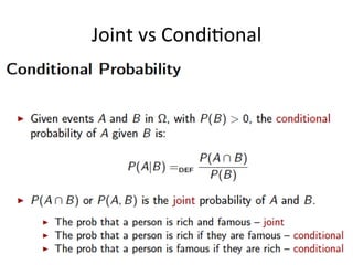
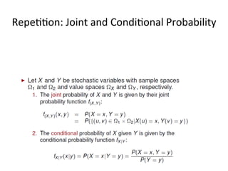
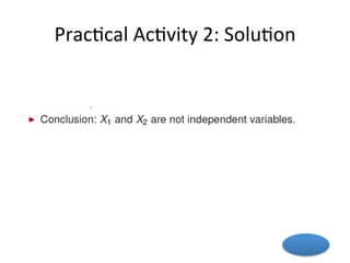
![Quiz
2:
Solu*ons
1. The
probability
is
0.1
—
incorrect
[We
cannot
compute
P(Dis|Sym)
from
P(Sym|Dis)
without
addi*onal
informa*on.]
2. The
probability
is
0.9
—
incorrect
[We
cannot
compute
P(Dis|Sym)
from
P(Sym|Dis)
without
addi*onal
informa*on.]
3. Nothing
—
correct
[We
cannot
compute
P(Dis|
Sym)
from
P(Sym|Dis)
without
addi*onal
informa*on.]
23](https://image.slidesharecdn.com/42jointmarginalconditionalprobmath4lt-150316083455-conversion-gate01/85/Lecture-Joint-Conditional-and-Marginal-Probabilities-23-320.jpg)


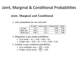
The document discusses joint, conditional, and marginal probabilities. It begins with an introduction to joint and conditional probabilities, defining conditional probability as the probability of event A given event B. It then presents the multiplication rule for calculating joint probabilities from conditional probabilities and marginal probabilities. The document provides examples and calculations to illustrate these probability concepts. It concludes with short quizzes to test understanding of applying the multiplication rule.