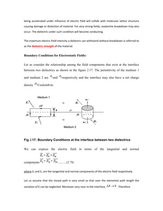
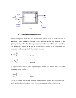
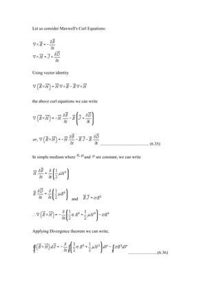
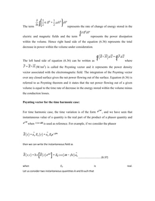
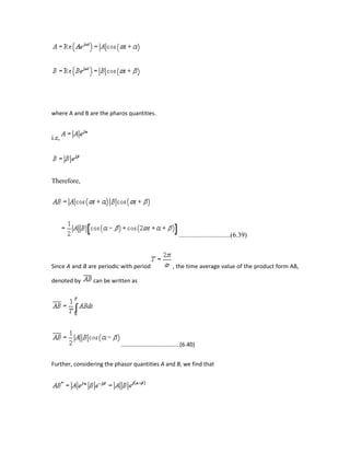
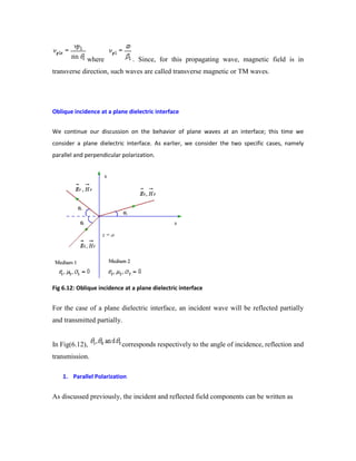
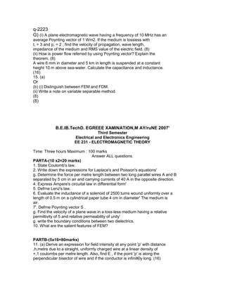
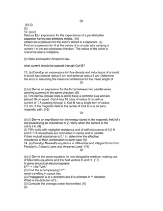
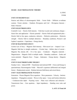
The document provides a comprehensive syllabus for the Electromagnetic Theory course, covering fundamental concepts, electrostatics, magnetostatics, electrodynamic fields, and electromagnetic waves. It includes detailed topics, textbooks, references, and highlights the significance of electromagnetic theory in electrical engineering and various fields. The curriculum aims to establish a solid understanding of vector calculus, field quantities, and the mathematical foundations crucial for analyzing electromagnetic phenomena.
![Sources of EMF:
Current carrying conductors.
Mobile phones.
Microwave oven.
Computer and Television screen.
High voltage Power lines.
Effects of Electromagnetic fields:
Plants and Animals.
Humans.
Electrical components.
Fields are classified as
Scalar field
Vector field.
Electric charge is a fundamental property of matter. Charge exist only in positive or
negative integral multiple of electronic charge, -e, e= 1.60 × 10⁻¹⁹
coulombs. [It may be
noted here that in 1962, Murray Gell-Mann hypothesized Quarks as the basic building
blocks of matters. Quarks were predicted to carry a fraction of electronic charge and the
existence of Quarks have been experimentally verified.] Principle of conservation of
charge states that the total charge (algebraic sum of positive and negative charges) of an
isolated system remains unchanged, though the charges may redistribute under the
influence of electric field. Kirchhoff's Current Law (KCL) is an assertion of the
conservative property of charges under the implicit assumption that there is no
accumulation of charge at the junction.](https://image.slidesharecdn.com/electromagnetictheory-140524093828-phpapp02/85/Electromagnetic-Theory-6-320.jpg)
![Electromagnetic theory deals directly with the electric and magnetic field vectors where as
circuit theory deals with the voltages and currents. Voltages and currents are integrated
effects of electric and magnetic fields respectively. Electromagnetic field problems involve
three space variables along with the time variable and hence the solution tends to become
correspondingly complex. Vector analysis is a mathematical tool with which electromagnetic
concepts are more conveniently expressed and best comprehended. Since use of vector
analysis in the study of electromagnetic field theory results in real economy of time and
thought, we first introduce the concept of vector analysis.
Vector Analysis:
The quantities that we deal in electromagnetic theory may be either scalar or vectors
[There are other class of physical quantities called Tensors: where magnitude and
direction vary with co ordinate axes]. Scalars are quantities characterized by magnitude
only and algebraic sign. A quantity that has direction as well as magnitude is called a
vector. Both scalar and vector quantities are function of time and position . A field is a
function that specifies a particular quantity everywhere in a region. Depending upon the
nature of the quantity under consideration, the field may be a vector or a scalar field.
Example of scalar field is the electric potential in a region while electric or magnetic
fields at any point is the example of vector field.
A vector can be written as, , where, is the magnitude and is the
unit vector which has unit magnitude and same direction as that of .
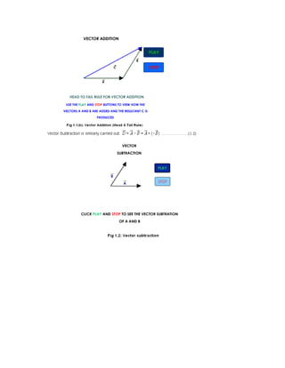
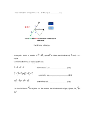
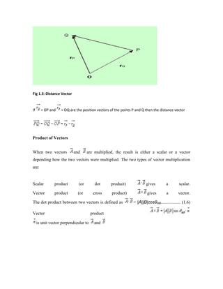
Two vector and are added together to give another vector . We have
................ (1.1)
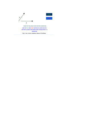
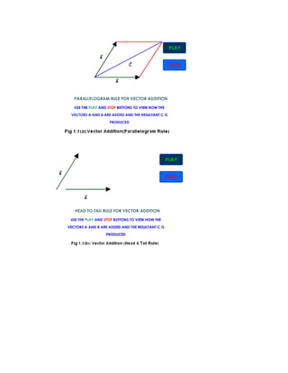
Let us see the animations in the next pages for the addition of two vectors, which has two
rules: 1: Parallelogram law and 2: Head & tail rule](https://image.slidesharecdn.com/electromagnetictheory-140524093828-phpapp02/85/Electromagnetic-Theory-7-320.jpg)