This document discusses the natural and step responses of parallel RLC circuits. It begins by presenting the governing differential equation and initial conditions for the voltage in a parallel RLC circuit. It then describes the three types of natural responses - overdamped, underdamped, and critically damped - based on the relationship between the neper and resonance frequencies. Examples are provided to demonstrate solving for the circuit parameters and determining the evolution of the voltage and branch currents over time for both overdamped and underdamped cases.

1. 1
Chapter 8
Natural and Step Responses of
RLC Circuits
8.1-2 The Natural Response of a Parallel RLC
Circuit
8.3 The Step Response of a Parallel RLC
Circuit
8.4 The Natural and Step Response of a
Series RLC Circuit

2. 2
Key points
 What do the response curves of over-, under-,
and critically-damped circuits look like? How to
choose R, L, C values to achieve fast switching
or to prevent overshooting damage?
 What are the initial conditions in an RLC circuit?
How to use them to determine the expansion
coefficients of the complete solution?
 Comparisons between: (1) natural & step
responses, (2) parallel, series, or general RLC.

3. 3
Section 8.1, 8.2
The Natural Response of a
Parallel RLC Circuit
1. ODE, ICs, general solution of parallel
voltage
2. Over-damped response
3. Under-damped response
4. Critically-damped response

4. 4
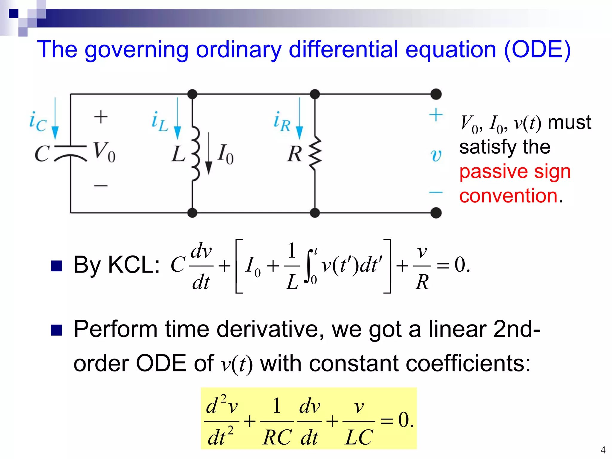
The governing ordinary differential equation (ODE)
.
0
)
(
1
0
0 






 


  R
v
t
d
t
v
L
I
dt
dv
C
t
 By KCL:
.
0
1
2
2



LC
v
dt
dv
RC
dt
v
d
 Perform time derivative, we got a linear 2nd-
order ODE of v(t) with constant coefficients:
V0, I0, v(t) must
satisfy the
passive sign
convention.

5. 5
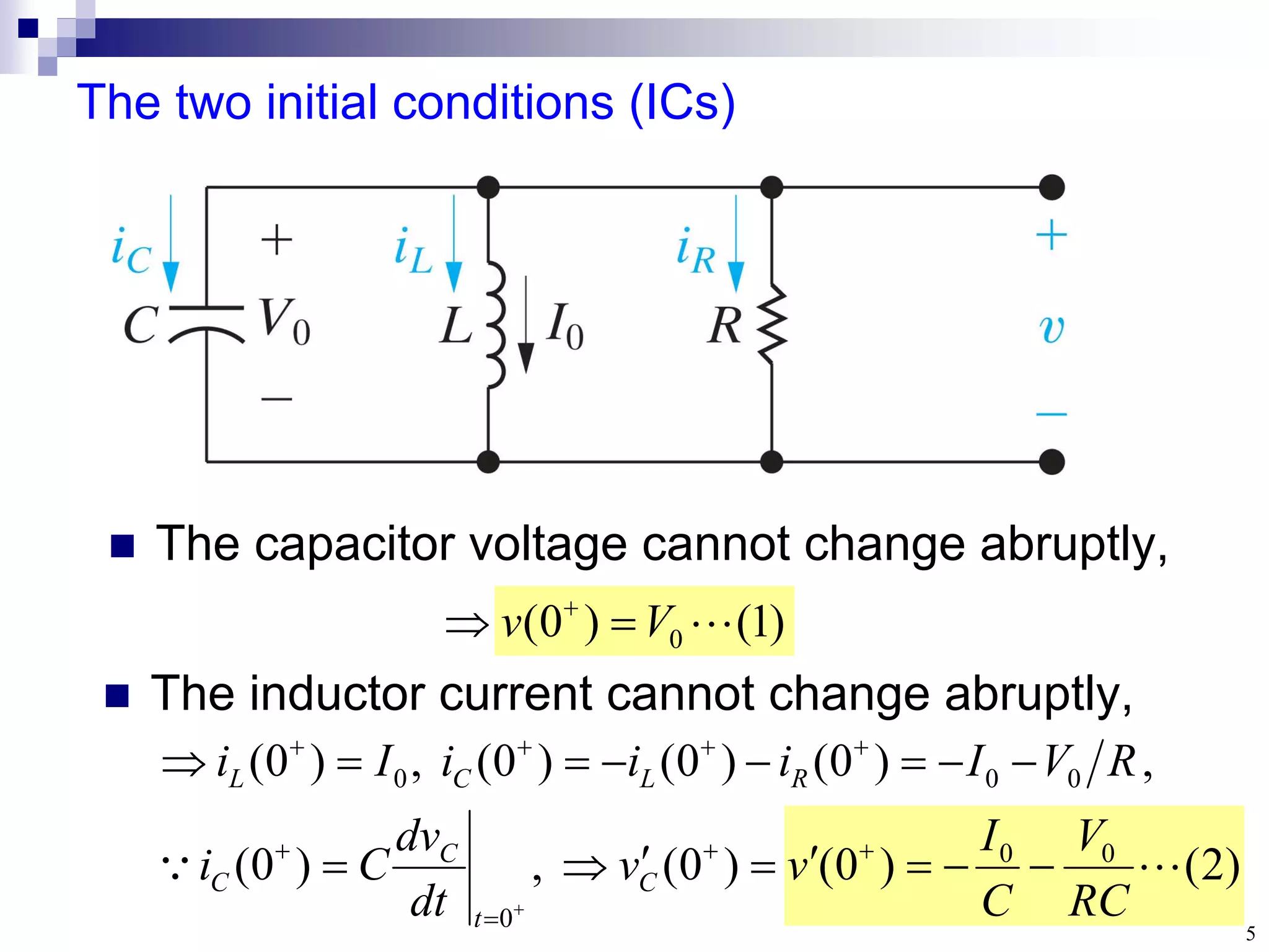
The two initial conditions (ICs)
 The capacitor voltage cannot change abruptly,
)
2
(
)
0
(
)
0
(
,
)
0
(
,
)
0
(
)
0
(
)
0
(
,
)
0
(
0
0
0
0
0
0


RC
V
C
I
v
v
dt
dv
C
i
R
V
I
i
i
i
I
i
C
t
C
C
R
L
C
L

























)
1
(
)
0
( 0 
V
v 
 
 The inductor current cannot change abruptly,

6. 6
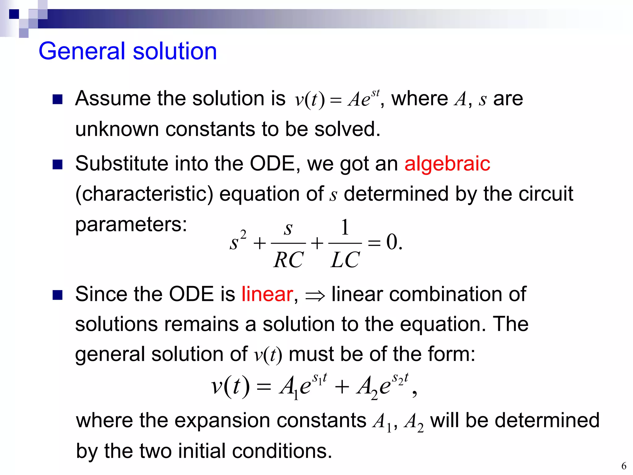
General solution
.
0
1
2



LC
RC
s
s
 Assume the solution is , where A, s are
unknown constants to be solved.
 Substitute into the ODE, we got an algebraic
(characteristic) equation of s determined by the circuit
parameters:
st
Ae
t
v 
)
(
where the expansion constants A1, A2 will be determined
by the two initial conditions.
,
)
( 2
1
2
1
t
s
t
s
e
A
e
A
t
v 

 Since the ODE is linear,  linear combination of
solutions remains a solution to the equation. The
general solution of v(t) must be of the form:

7. 7
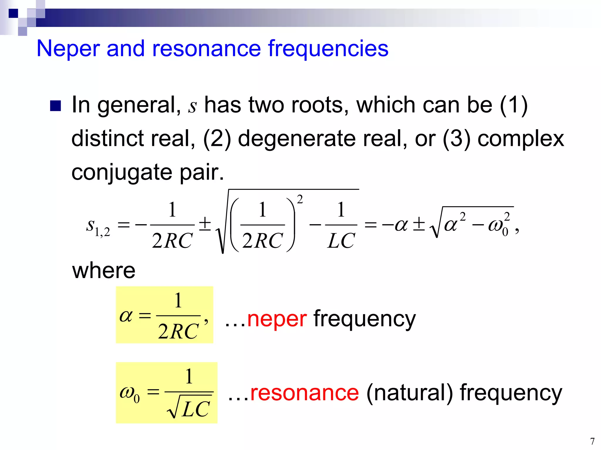
Neper and resonance frequencies
 In general, s has two roots, which can be (1)
distinct real, (2) degenerate real, or (3) complex
conjugate pair.
,
1
2
1
2
1 2
0
2
2
2
,
1 

 













LC
RC
RC
s
LC
1
0 

,
2
1
RC


where
…resonance (natural) frequency
…neper frequency

8. 8
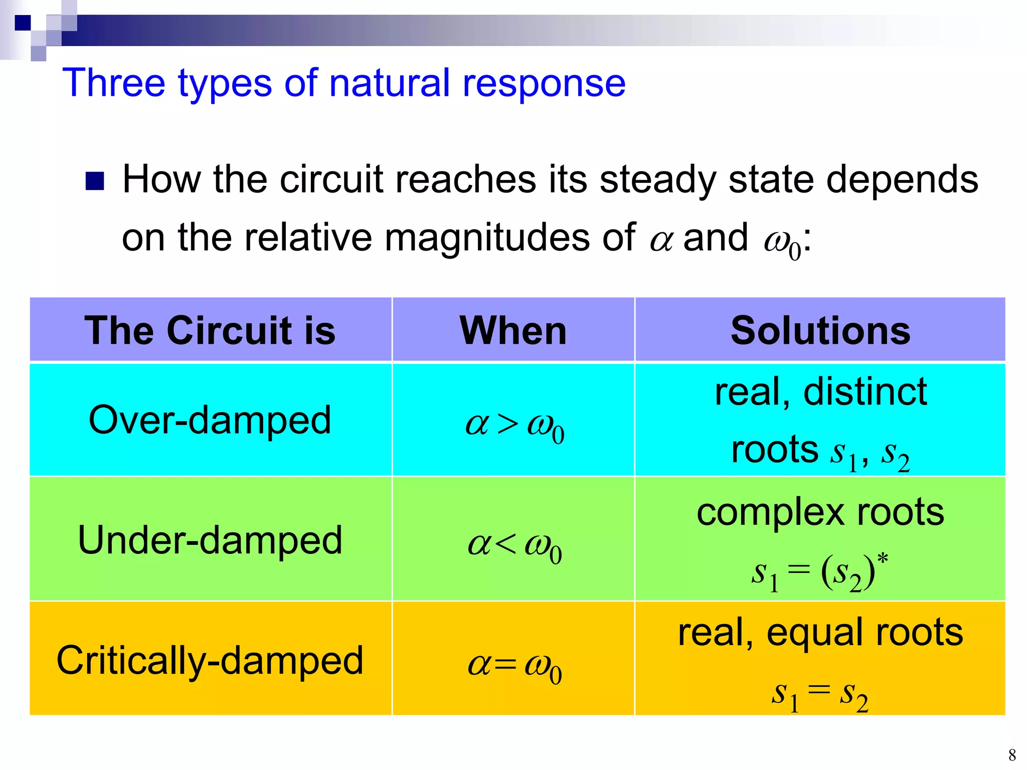
Three types of natural response
Over-damped  
real, distinct
roots s1, s2
Under-damped 
complex roots
s1 = (s2)*
Critically-damped 
real, equal roots
s1 = s2
The Circuit is When Solutions
 How the circuit reaches its steady state depends
on the relative magnitudes of  and 0:

9. 9
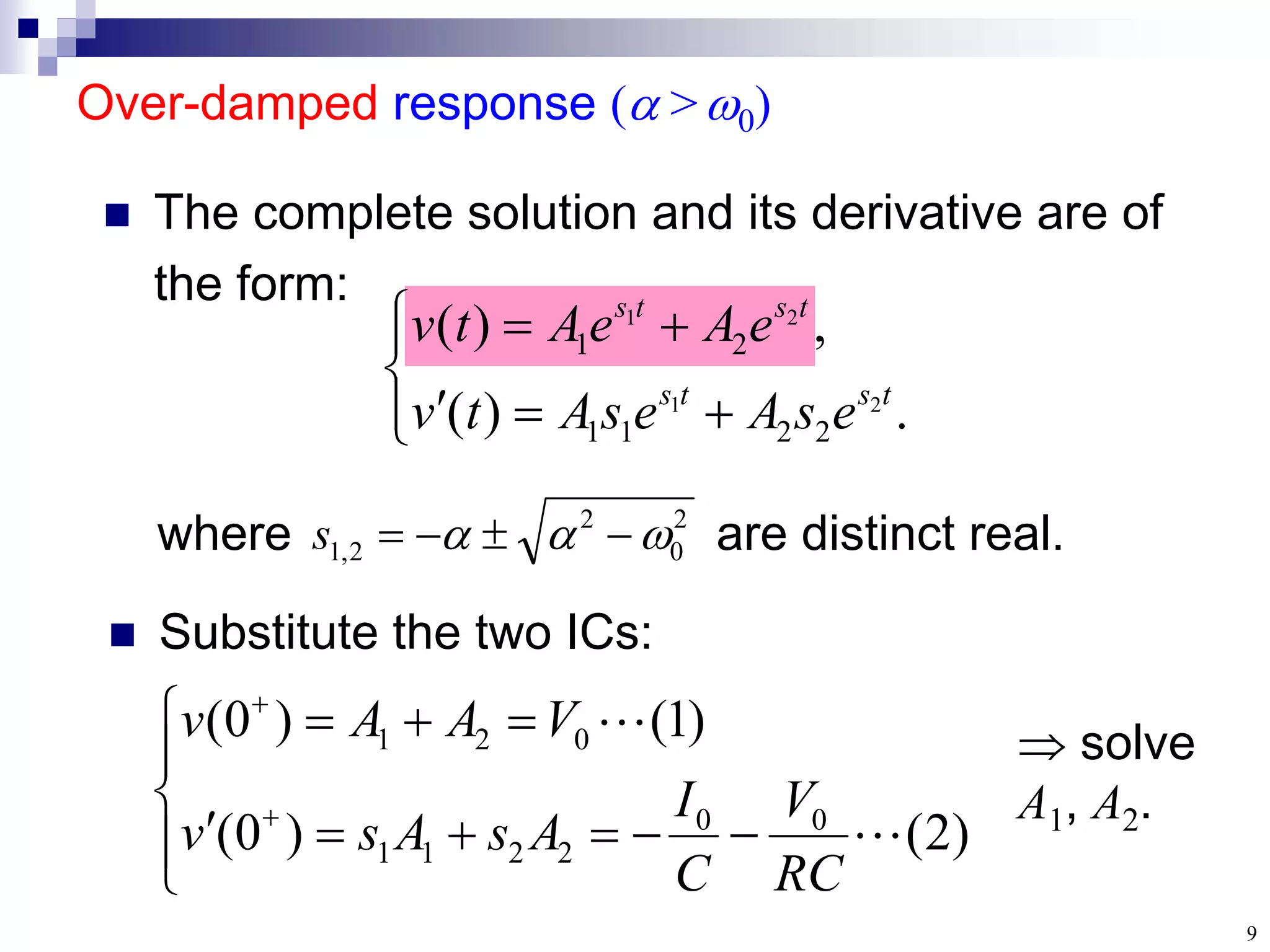
where are distinct real.
Over-damped response ( >0)
 The complete solution and its derivative are of
the form:










.
)
(
,
)
(
2
1
2
1
2
2
1
1
2
1
t
s
t
s
t
s
t
s
e
s
A
e
s
A
t
v
e
A
e
A
t
v
2
0
2
2
,
1 

 



s
 Substitute the two ICs:
















)
2
(
)
0
(
)
1
(
)
0
(
0
0
2
2
1
1
0
2
1


RC
V
C
I
A
s
A
s
v
V
A
A
v  solve
A1, A2.

10. 10
Example 8.2: Discharging a parallel RLC circuit (1)
12 V 30 mA
 Q: v(t), iC(t), iL(t), iR(t)=?



















kHz.
10
)
10
2
)(
10
5
(
1
1
,
kHz
5
.
12
)
10
2
)(
200
(
2
1
2
1
7
2
0
7
LC
RC

  >0,
over-
damped

11. 11
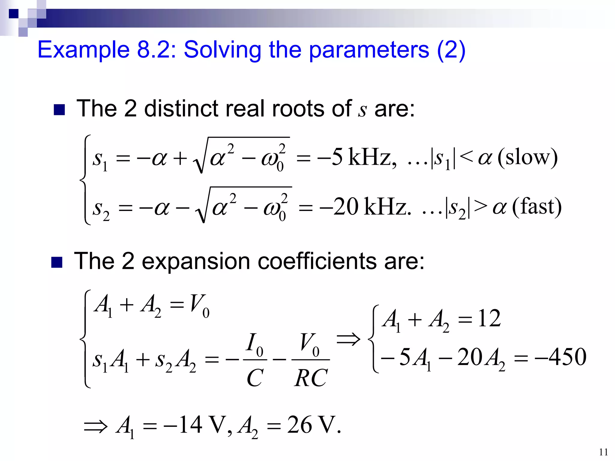
Example 8.2: Solving the parameters (2)
 The 2 distinct real roots of s are:

















.
kHz
20
,
kHz
5
2
0
2
2
2
0
2
1






s
s
…|s2|>(fast)
…|s1|<(slow)





















450
20
5
12
2
1
2
1
0
0
2
2
1
1
0
2
1
A
A
A
A
RC
V
C
I
A
s
A
s
V
A
A
 The 2 expansion coefficients are:
V.
26
,
V
14 2
1 


 A
A

12. 12
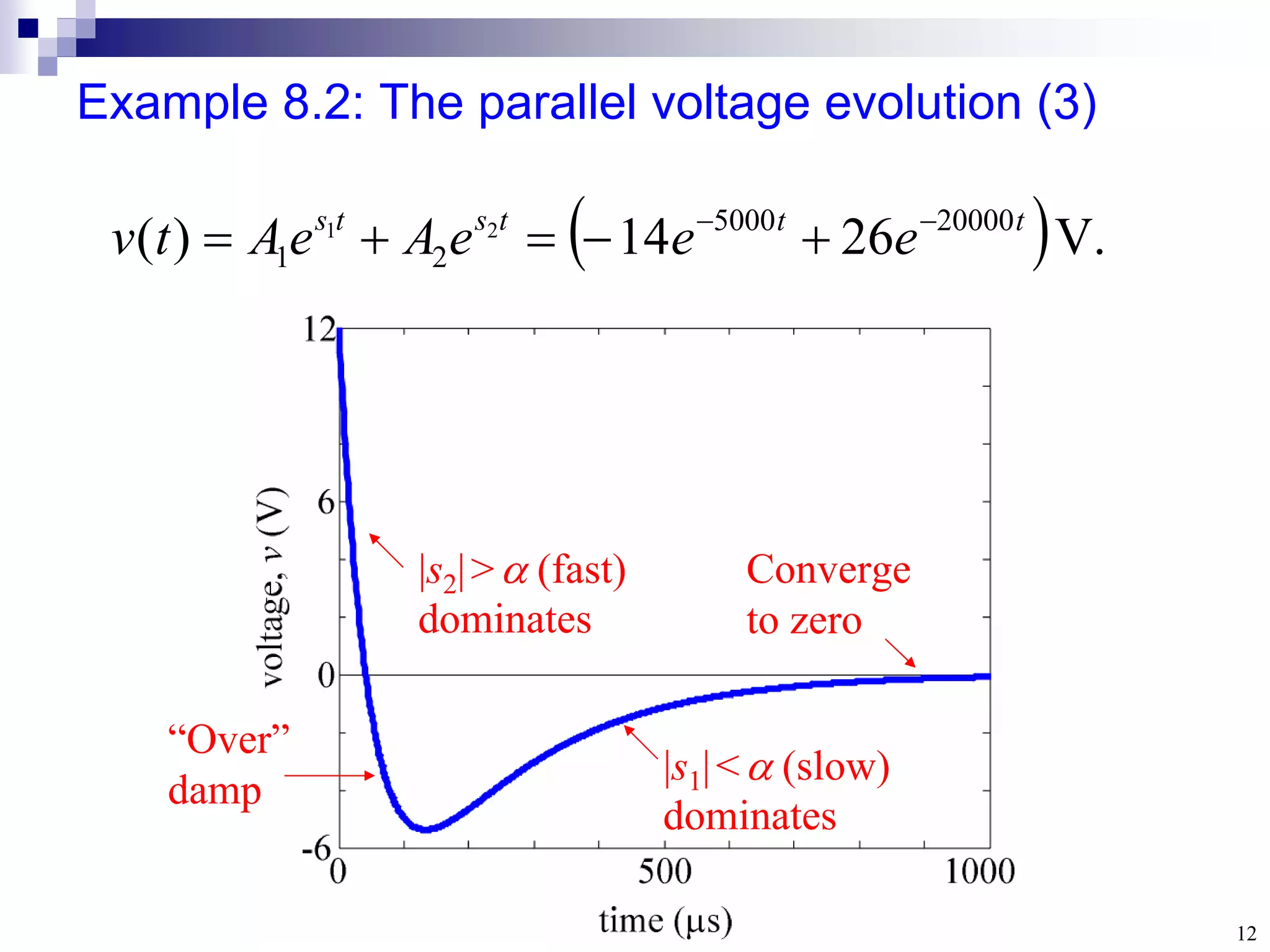
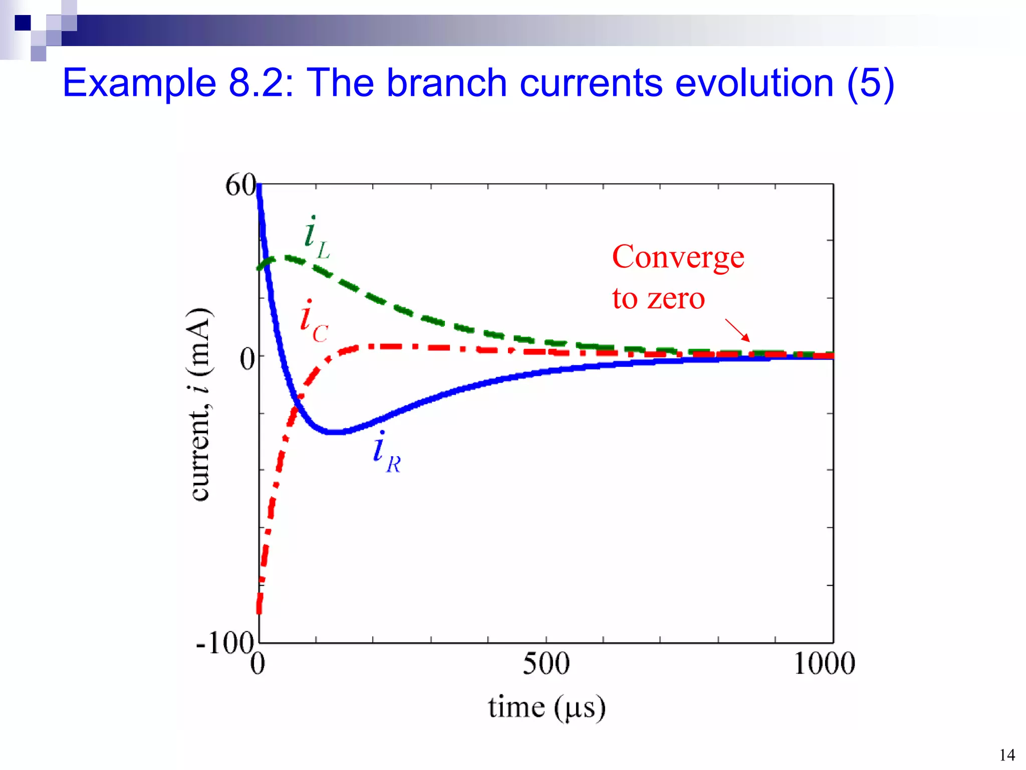
Example 8.2: The parallel voltage evolution (3)
Converge
to zero
|s1|<(slow)
dominates
|s2|>(fast)
dominates
 V.
26
14
)
( 20000
5000
2
1
2
1 t
t
t
s
t
s
e
e
e
A
e
A
t
v 






“Over”
damp

13. 13
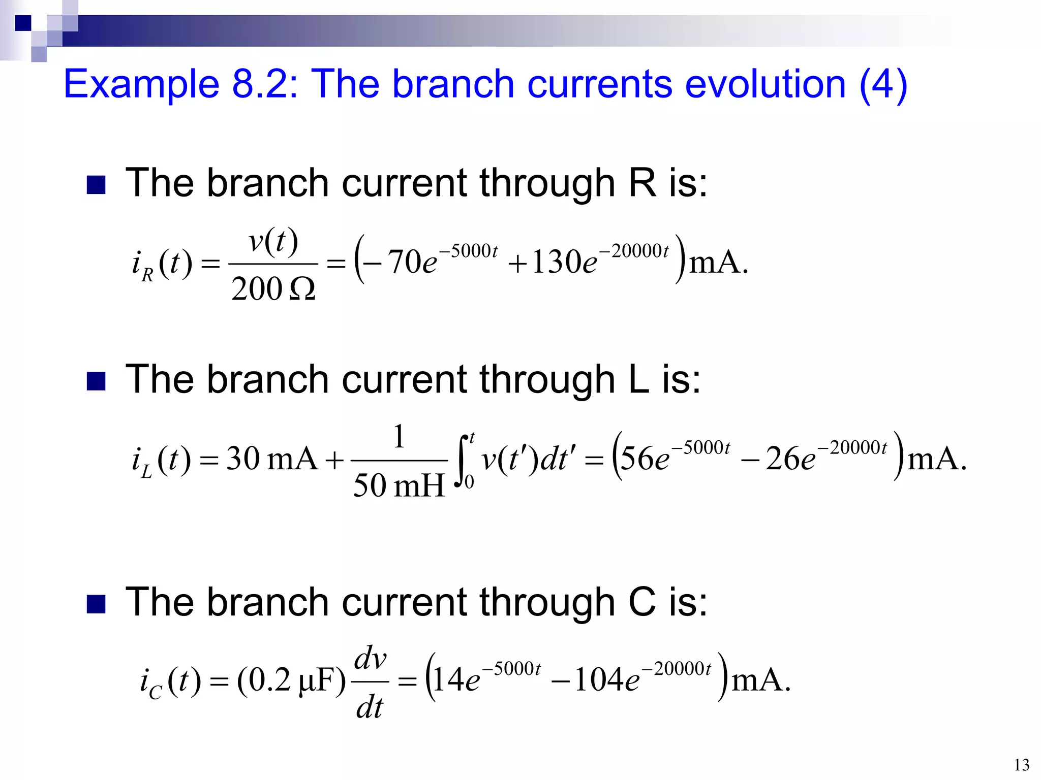
Example 8.2: The branch currents evolution (4)
 The branch current through R is:
 mA.
130
70
200
)
(
)
( 20000
5000 t
t
R e
e
t
v
t
i 






 The branch current through L is:
 mA.
26
56
)
(
mH
0
5
1
mA
30
)
( 20000
5000
0
t
t
t
L e
e
t
d
t
v
t
i 






 
 The branch current through C is:
 mA.
104
14
μF)
2
.
0
(
)
( 20000
5000 t
t
C e
e
dt
dv
t
i 





14. 14
Example 8.2: The branch currents evolution (5)
Converge
to zero

15. 15
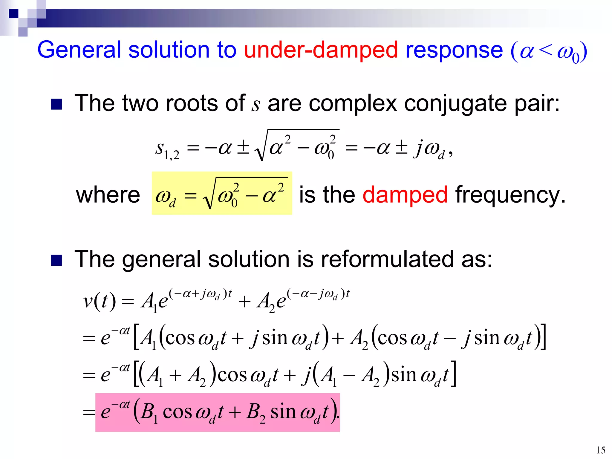
where is the damped frequency.
General solution to under-damped response ( <0)
 The two roots of s are complex conjugate pair:
2
2
0 

 

d
,
2
0
2
2
,
1 d
j
s 



 






   
 
   
 
 .
sin
cos
sin
cos
sin
cos
sin
cos
)
(
2
1
2
1
2
1
2
1
)
(
2
)
(
1
t
B
t
B
e
t
A
A
j
t
A
A
e
t
j
t
A
t
j
t
A
e
e
A
e
A
t
v
d
d
t
d
d
t
d
d
d
d
t
t
j
t
j d
d


































 The general solution is reformulated as:

16. 16
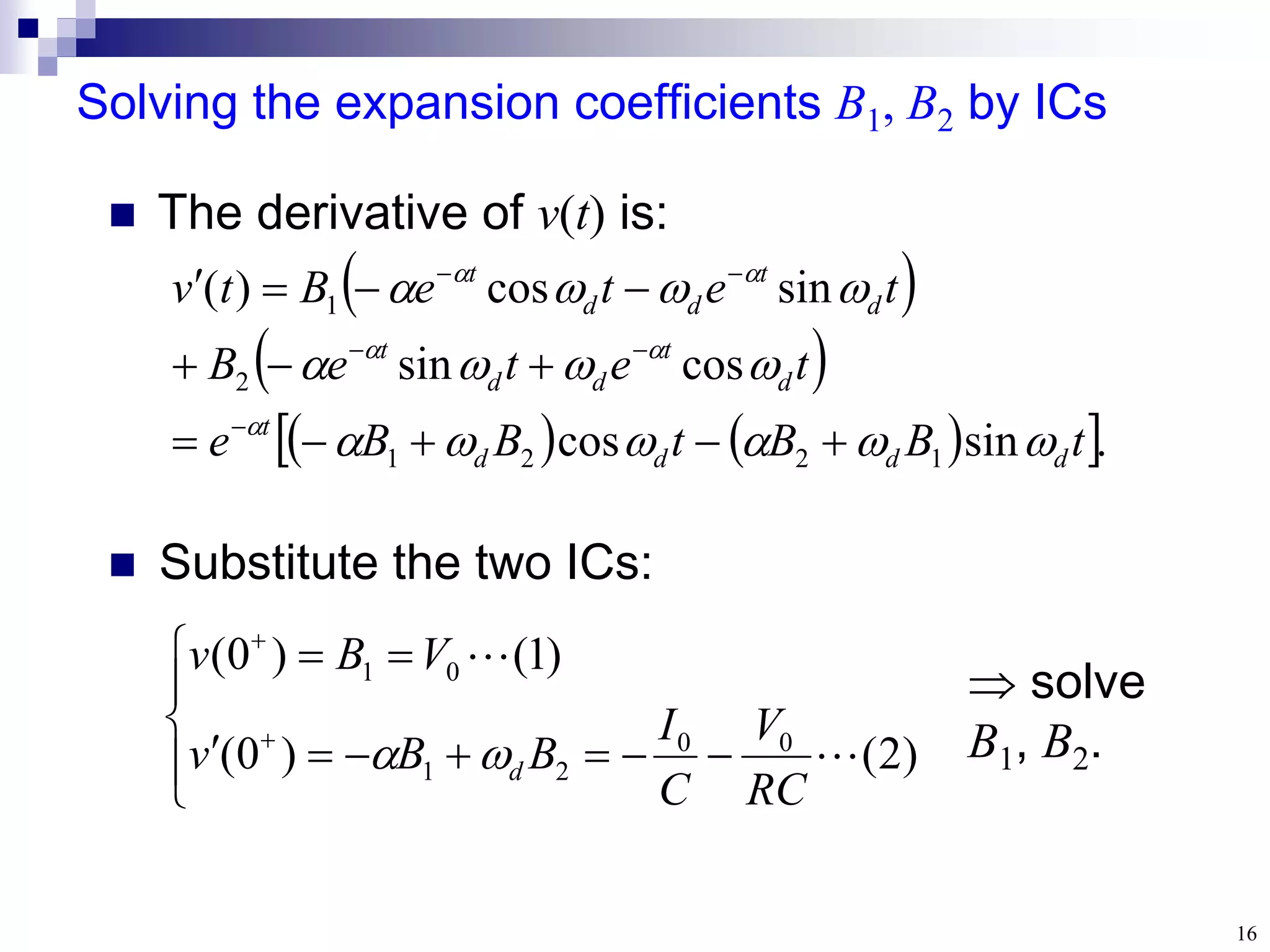
Solving the expansion coefficients B1, B2 by ICs
 Substitute the two ICs:
















)
2
(
)
0
(
)
1
(
)
0
(
0
0
2
1
0
1


RC
V
C
I
B
B
v
V
B
v
d


 solve
B1, B2.
 
 
   
 .
sin
cos
cos
sin
sin
cos
)
(
1
2
2
1
2
1
t
B
B
t
B
B
e
t
e
t
e
B
t
e
t
e
B
t
v
d
d
d
d
t
d
t
d
d
t
d
t
d
d
t




































 The derivative of v(t) is:

17. 17
Example 8.4: Discharging a parallel RLC circuit (1)
0 V
-12.25 mA
 Q: v(t), iC(t), iL(t), iR(t)=?


















kHz.
1
)
10
25
.
1
)(
8
(
1
1
,
kHz
2
.
0
)
10
25
.
1
)(
10
2
(
2
1
2
1
7
0
7
4
LC
RC

  <0,
under-
damped

18. 18
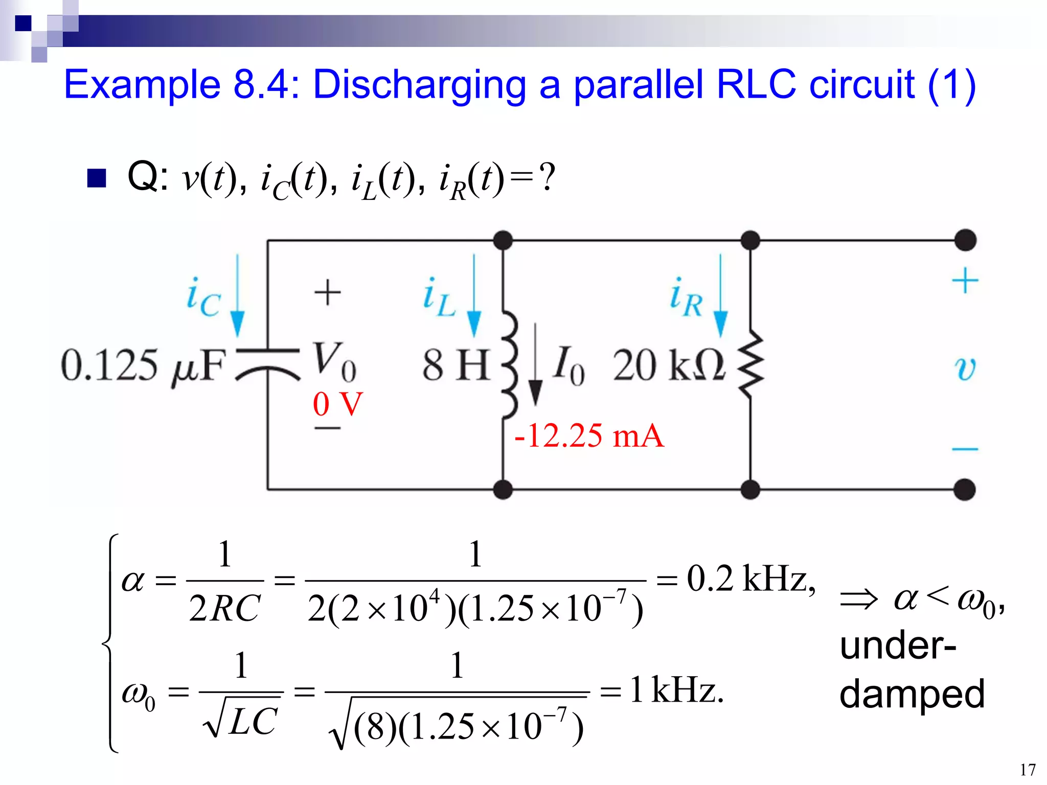
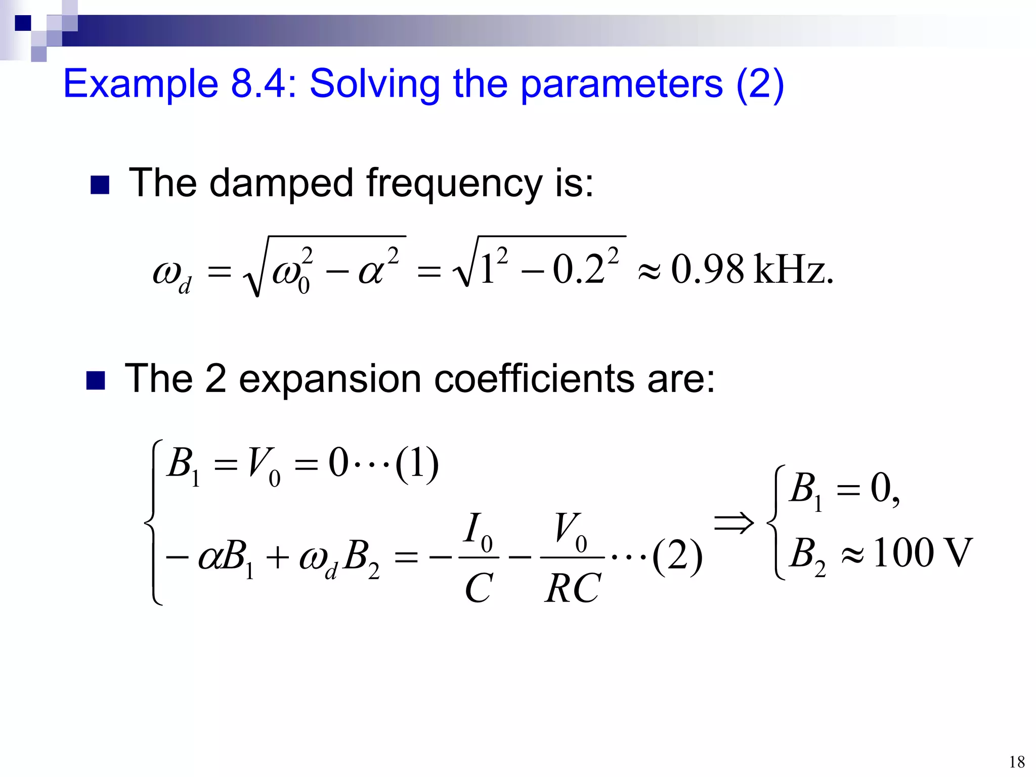
Example 8.4: Solving the parameters (2)
.
kHz
98
.
0
2
.
0
1 2
2
2
2
0 



 

d
 The damped frequency is:
 The 2 expansion coefficients are:


















V
100
,
0
)
2
(
)
1
(
0
2
1
0
0
2
1
0
1
B
B
RC
V
C
I
B
B
V
B
d 




19. 19
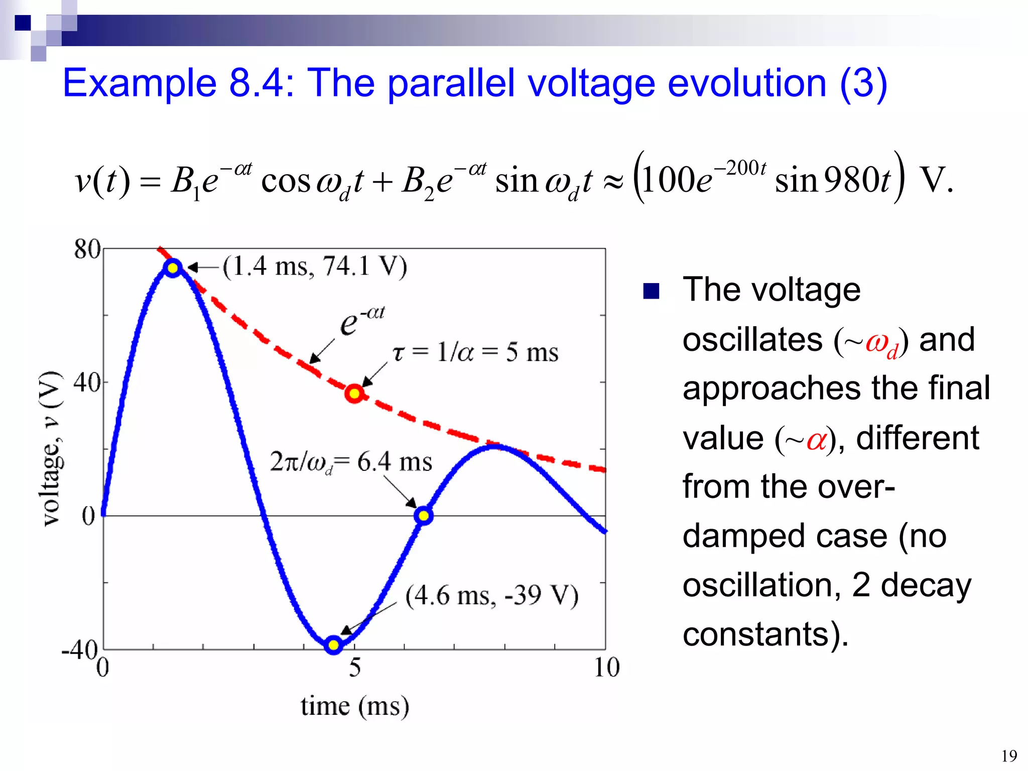
Example 8.4: The parallel voltage evolution (3)
  .
V
980
sin
100
sin
cos
)
( 200
2
1 t
e
t
e
B
t
e
B
t
v t
d
t
d
t 




 
 

 The voltage
oscillates (~d) and
approaches the final
value (~), different
from the over-
damped case (no
oscillation, 2 decay
constants).

20. 20
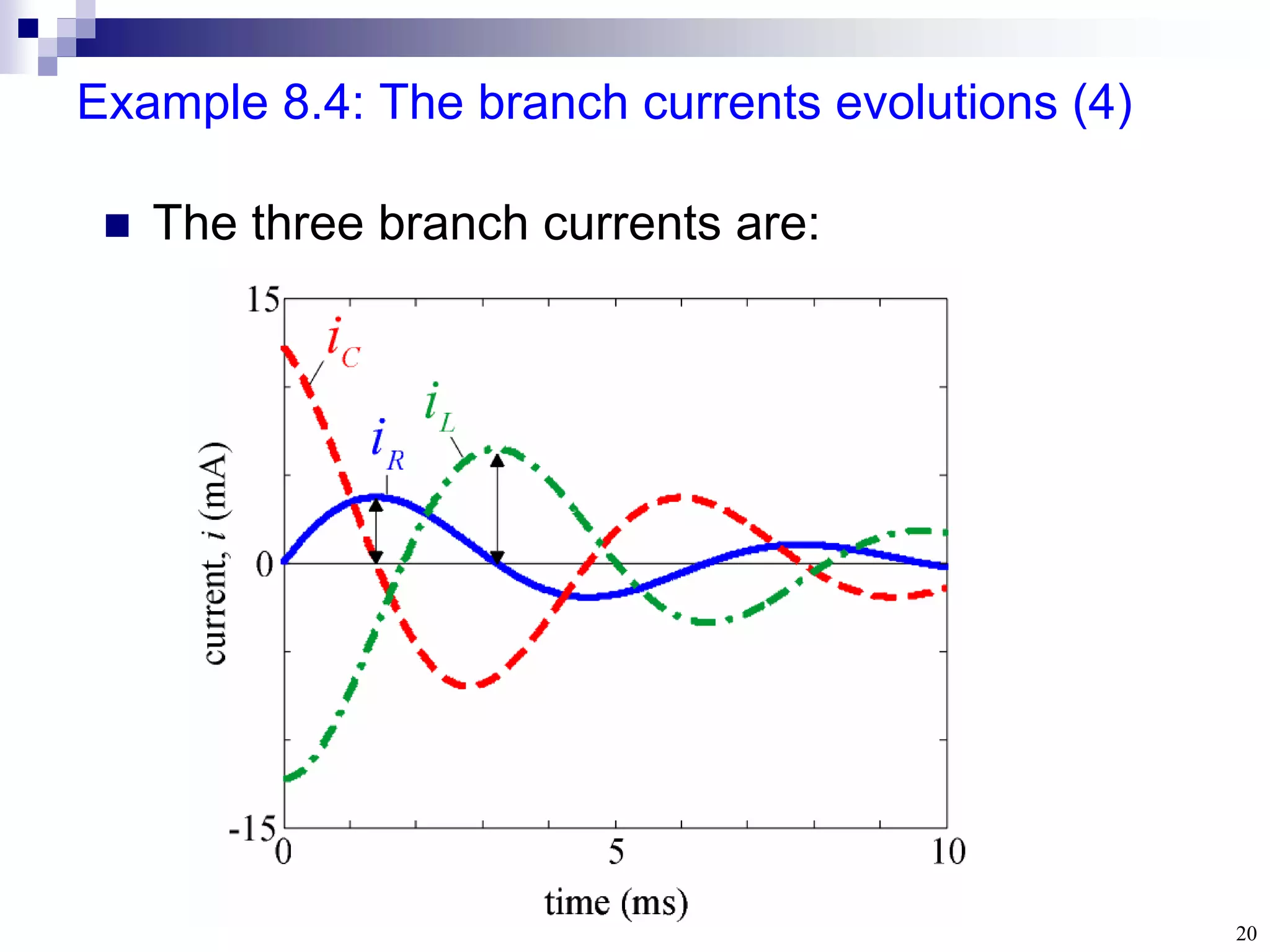
Example 8.4: The branch currents evolutions (4)
 The three branch currents are:

21. 21
Rules for circuit designers
 If one desires the circuit reaches the final value
as fast as possible while the minor oscillation is
of less concern, choosing R, L, C values to
satisfy under-damped condition.
 If one concerns that the response not exceed its
final value to prevent potential damage,
designing the system to be over-damped at the
cost of slower response.

22. 22
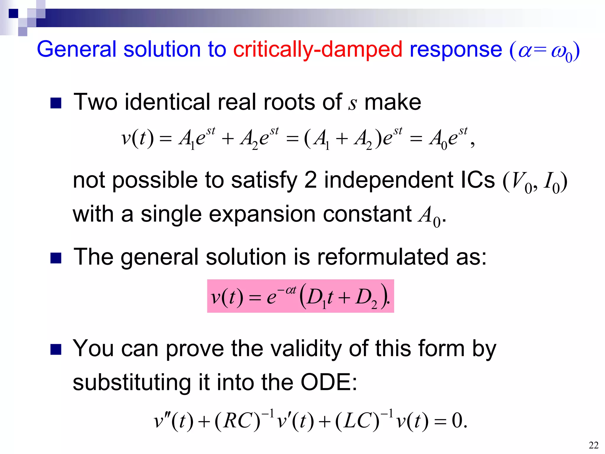
General solution to critically-damped response (=0)
 Two identical real roots of s make
 The general solution is reformulated as:
,
)
(
)
( 0
2
1
2
1
st
st
st
st
e
A
e
A
A
e
A
e
A
t
v 




not possible to satisfy 2 independent ICs (V0, I0)
with a single expansion constant A0.
 .
)
( 2
1 D
t
D
e
t
v t

 
 You can prove the validity of this form by
substituting it into the ODE:
.
0
)
(
)
(
)
(
)
(
)
( 1
1





 

t
v
LC
t
v
RC
t
v

23. 23
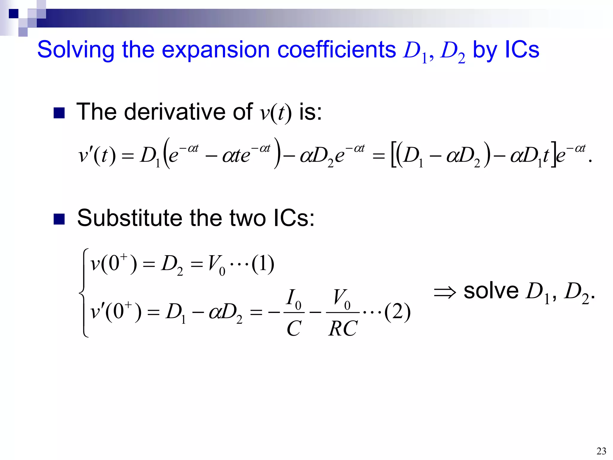
Solving the expansion coefficients D1, D2 by ICs
 Substitute the two ICs:















)
2
(
)
0
(
)
1
(
)
0
(
0
0
2
1
0
2


RC
V
C
I
D
D
v
V
D
v

 solve D1, D2.
   
  .
)
( 1
2
1
2
1
t
t
t
t
e
t
D
D
D
e
D
te
e
D
t
v 






 










 The derivative of v(t) is:

24. 24
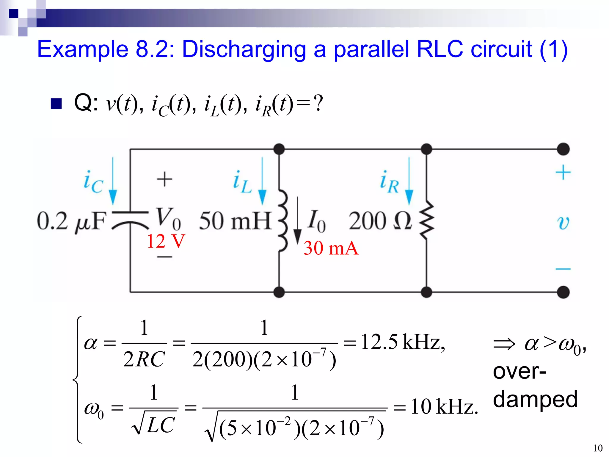
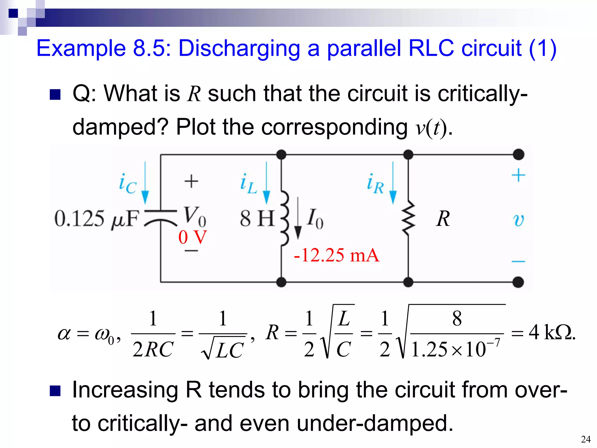
Example 8.5: Discharging a parallel RLC circuit (1)
0 V
-12.25 mA
R
 Q: What is R such that the circuit is critically-
damped? Plot the corresponding v(t).
.
k
4
10
25
.
1
8
2
1
2
1
,
1
2
1
, 7
0 





 
C
L
R
LC
RC


 Increasing R tends to bring the circuit from over-
to critically- and even under-damped.

25. 25
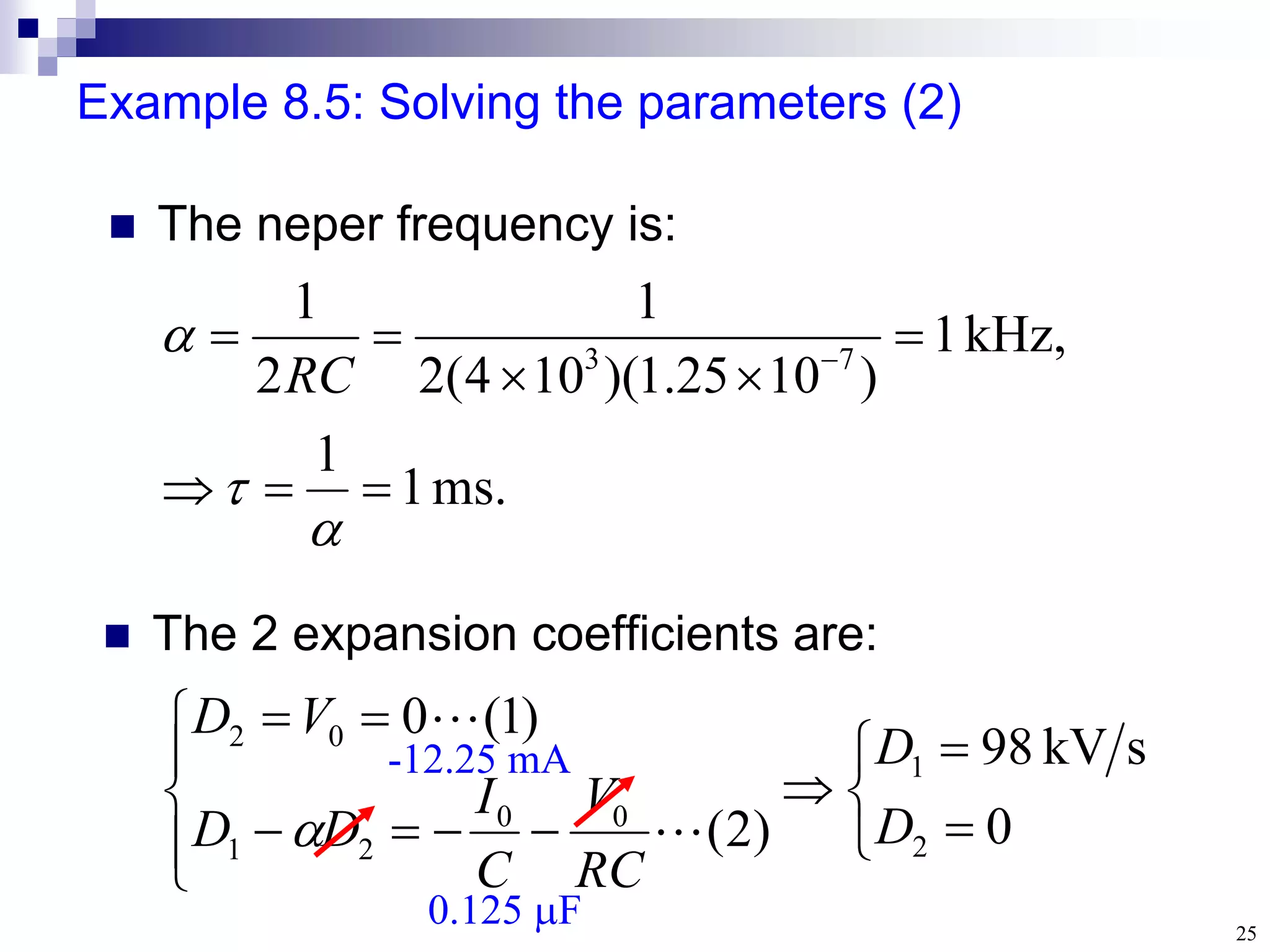
Example 8.5: Solving the parameters (2)
 The neper frequency is:
 The 2 expansion coefficients are:
ms.
1
1
,
kHz
1
)
10
25
.
1
)(
10
4
(
2
1
2
1
7
3







 



RC

















0
s
kV
98
)
2
(
)
1
(
0
2
1
0
0
2
1
0
2
D
D
RC
V
C
I
D
D
V
D



-12.25 mA
0.125 F

26. 26
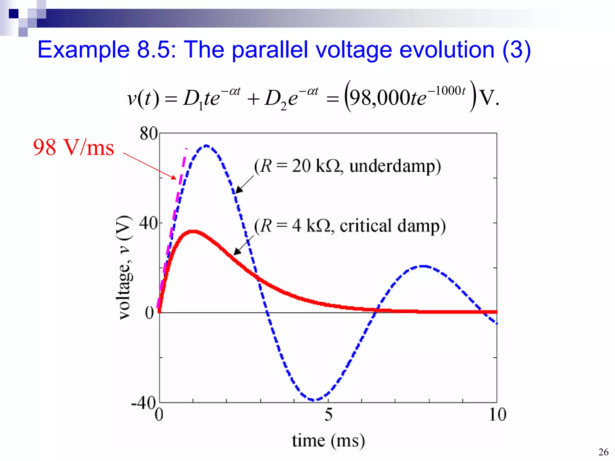
Example 8.5: The parallel voltage evolution (3)
98 V/ms
  .
V
000
,
98
)
( 1000
2
1
t
t
t
te
e
D
te
D
t
v 




 


27. 27
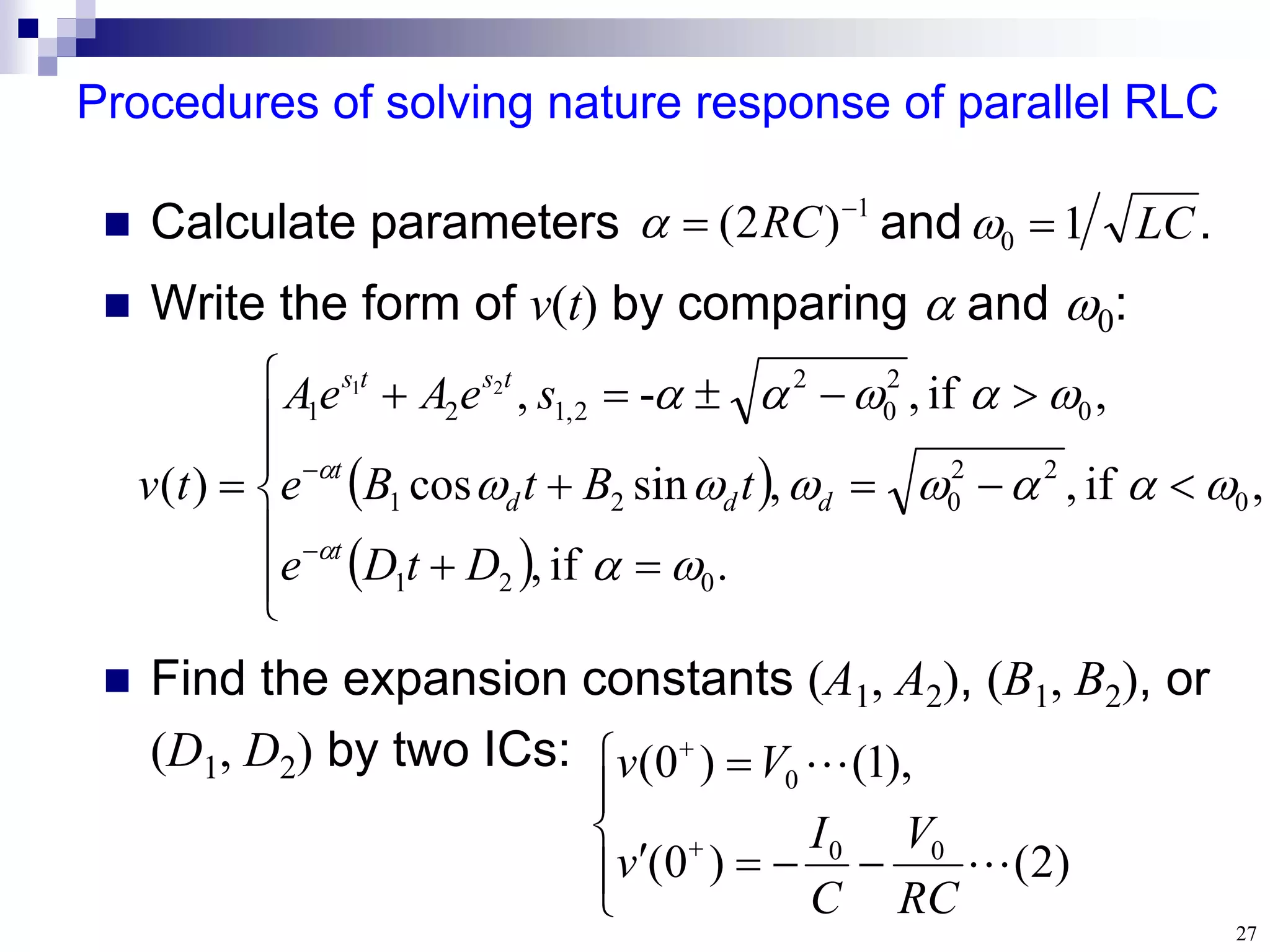
Procedures of solving nature response of parallel RLC
 Calculate parameters and .
 Write the form of v(t) by comparing  and :
 Find the expansion constants (A1, A2), (B1, B2), or
(D1, D2) by two ICs:
LC
1
0 

1
)
2
( 
 RC













)
2
(
)
0
(
),
1
(
)
0
(
0
0
0


RC
V
C
I
v
V
v
 
 





















.
if
,
,
if
,
,
sin
cos
,
if
,
-
,
)
(
0
2
1
0
2
2
0
2
1
0
2
0
2
2
,
1
2
1
2
1
















D
t
D
e
t
B
t
B
e
s
e
A
e
A
t
v
t
d
d
d
t
t
s
t
s

28. 28
Section 8.3
The Step Response of
a Parallel RLC Circuit
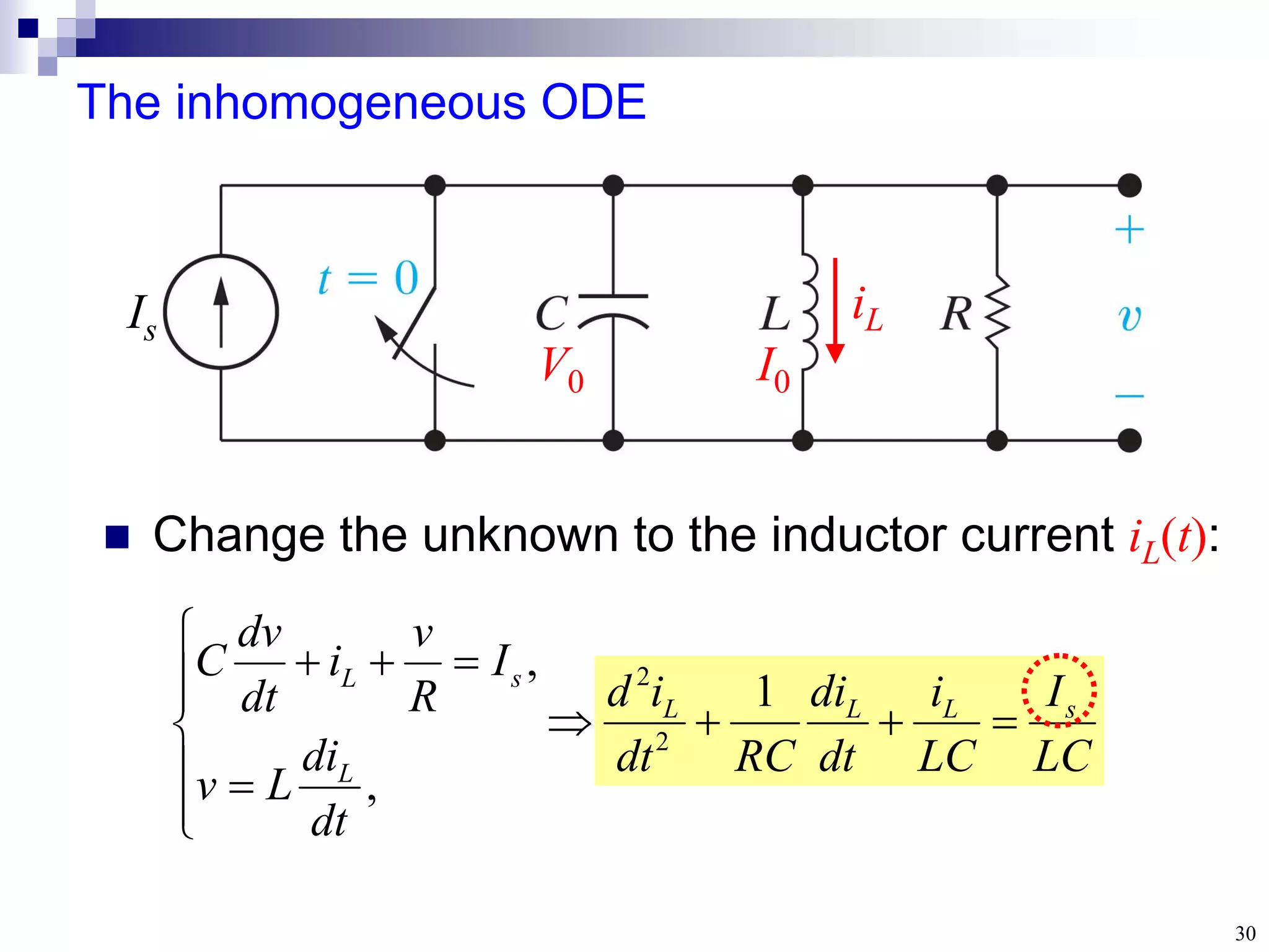
1. Inhomogeneous ODE, ICs, and general
solution

29. 29
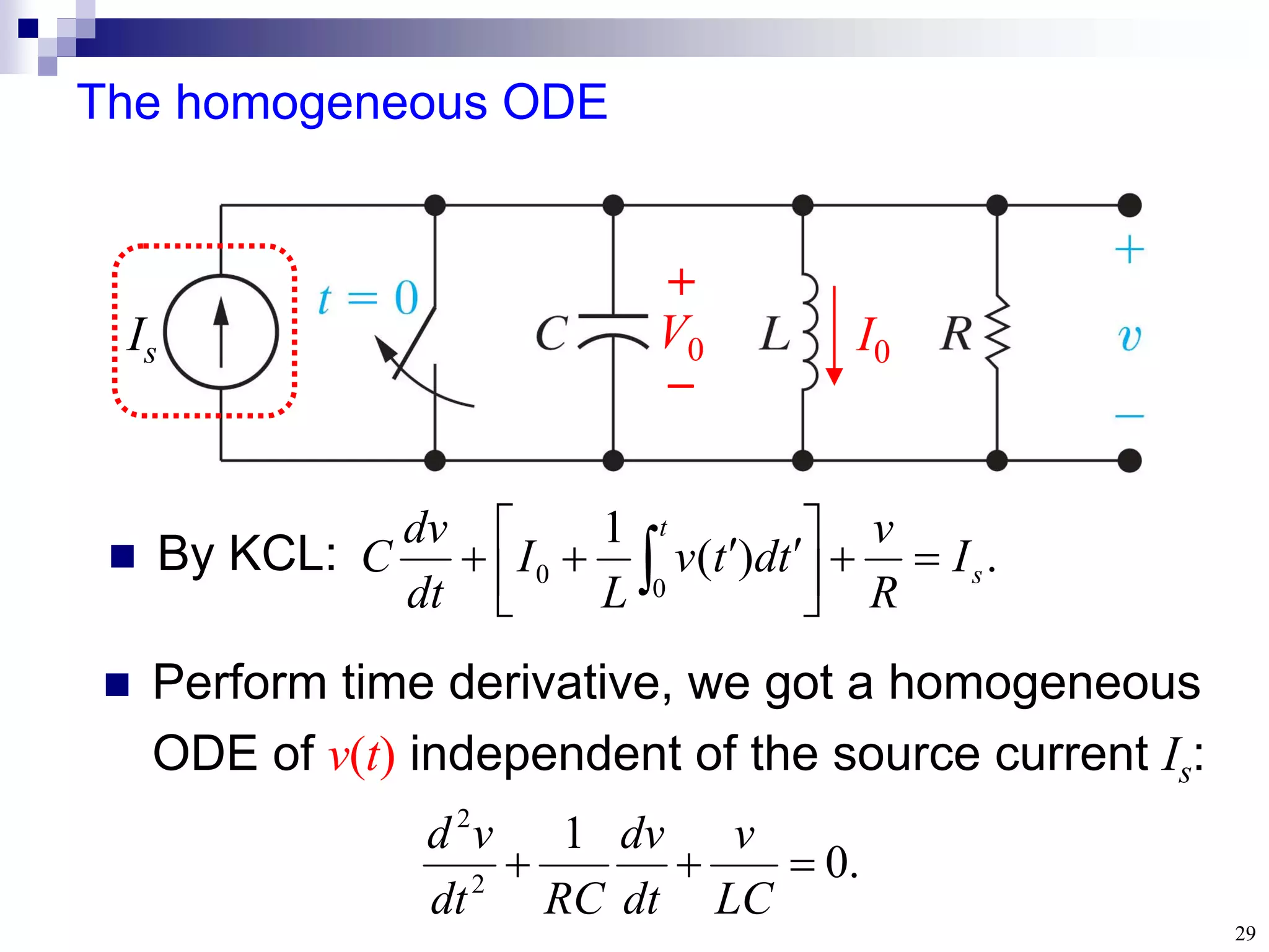
The homogeneous ODE
.
)
(
1
0
0 s
t
I
R
v
t
d
t
v
L
I
dt
dv
C 






 


 
 By KCL:
.
0
1
2
2



LC
v
dt
dv
RC
dt
v
d
 Perform time derivative, we got a homogeneous
ODE of v(t) independent of the source current Is:
V0 I0
Is
+


30. 30
The inhomogeneous ODE
LC
I
LC
i
dt
di
RC
dt
i
d
dt
di
L
v
I
R
v
i
dt
dv
C
s
L
L
L
L
s
L















1
,
,
2
2
 Change the unknown to the inductor current iL(t):
iL
V0 I0
Is

31. 31
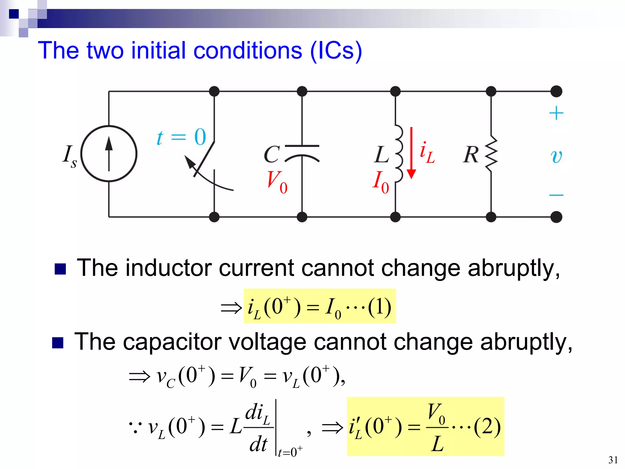
The two initial conditions (ICs)
 The inductor current cannot change abruptly,
)
2
(
)
0
(
,
)
0
(
),
0
(
)
0
(
0
0
0


L
V
i
dt
di
L
v
v
V
v
L
t
L
L
L
C













)
1
(
)
0
( 0 
I
iL 
 
 The capacitor voltage cannot change abruptly,
Is
iL
V0 I0

32. 32
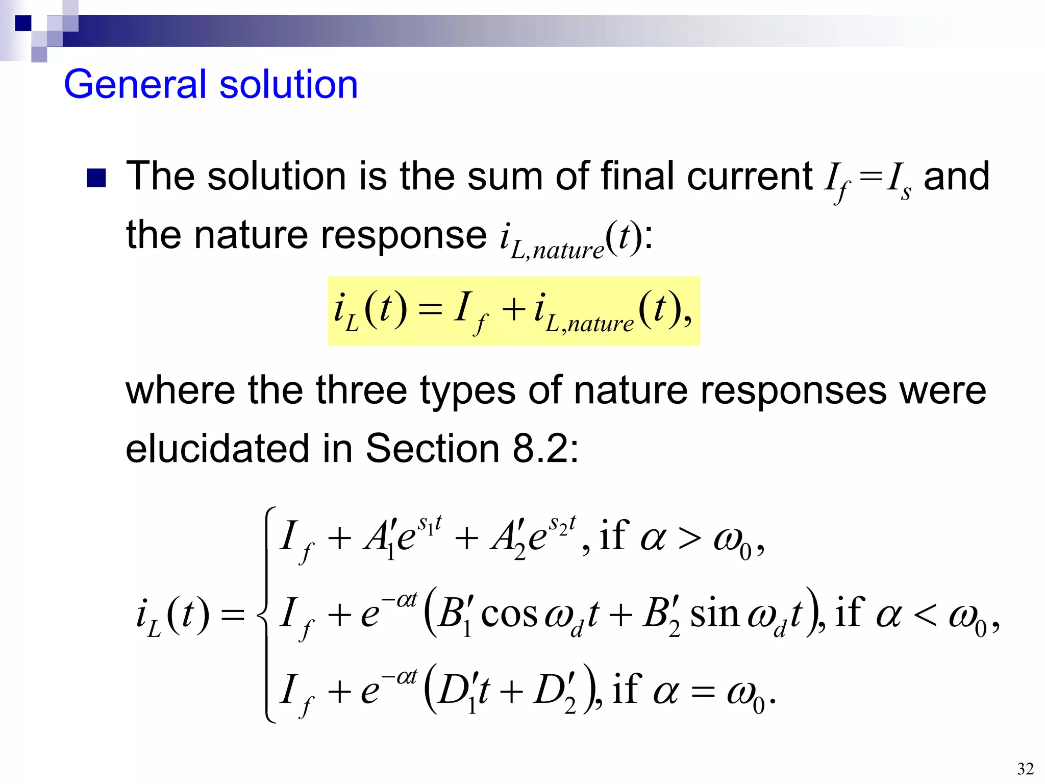
General solution
where the three types of nature responses were
elucidated in Section 8.2:
 The solution is the sum of final current If =Is and
the nature response iL,nature(t):
),
(
)
( , t
i
I
t
i nature
L
f
L 

 
 

























.
if
,
,
if
,
sin
cos
,
if
,
)
(
0
2
1
0
2
1
0
2
1
2
1










D
t
D
e
I
t
B
t
B
e
I
e
A
e
A
I
t
i
t
f
d
d
t
f
t
s
t
s
f
L

33. 33
Example 8.7: Charging a parallel RLC circuit (1)
625 
Is=
24
mA V0 =0
I0=0
 Q: iL(t) = ?



















kHz.
40
)
10
5
.
2
)(
10
5
.
2
(
1
1
,
kHz
32
)
10
5
.
2
)(
625
(
2
1
2
1
8
2
0
8
LC
RC

  <0,
under-
damped

34. 34
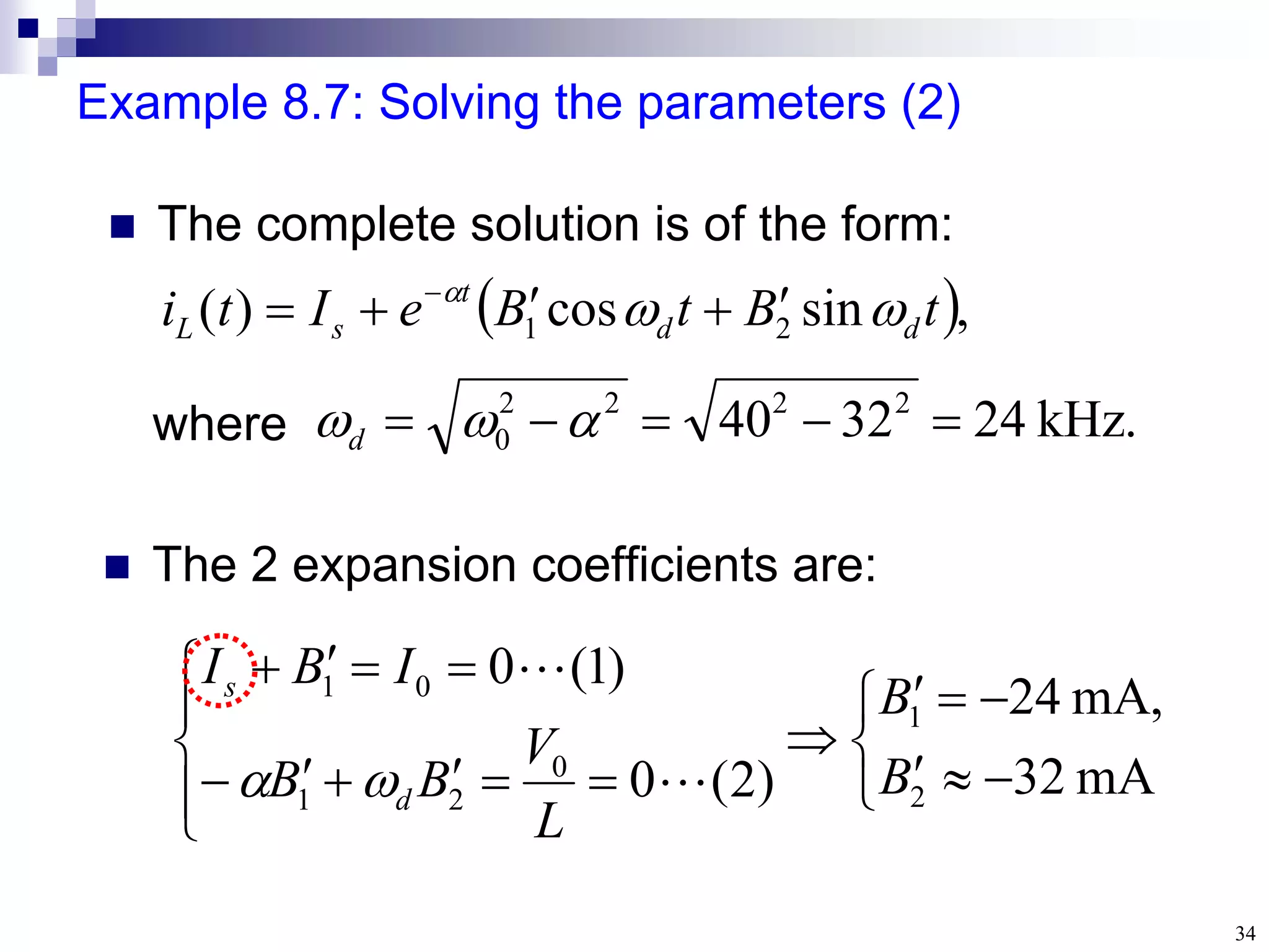
Example 8.7: Solving the parameters (2)
.
kHz
24
32
40 2
2
2
2
0 



 

d
 The complete solution is of the form:
 The 2 expansion coefficients are:

























mA
32
,
mA
24
)
2
(
0
)
1
(
0
2
1
0
2
1
0
1
B
B
L
V
B
B
I
B
I
d
s




 ,
sin
cos
)
( 2
1 t
B
t
B
e
I
t
i d
d
t
s
L 






 
where

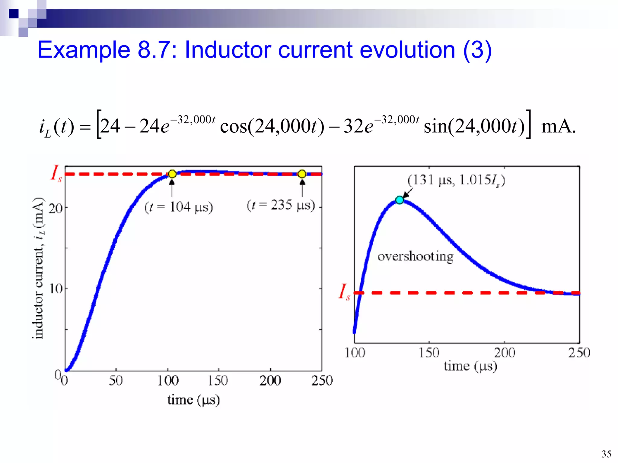
35. 35
Example 8.7: Inductor current evolution (3)
  .
mA
)
000
,
24
sin(
32
)
000
,
24
cos(
24
24
)
( 000
,
32
000
,
32
t
e
t
e
t
i t
t
L






36. 36
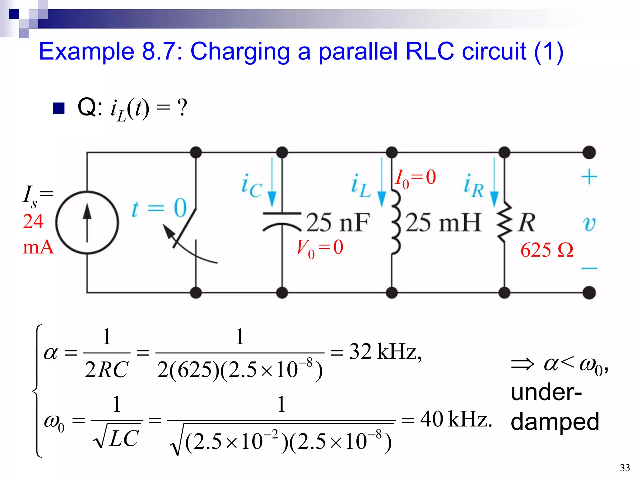
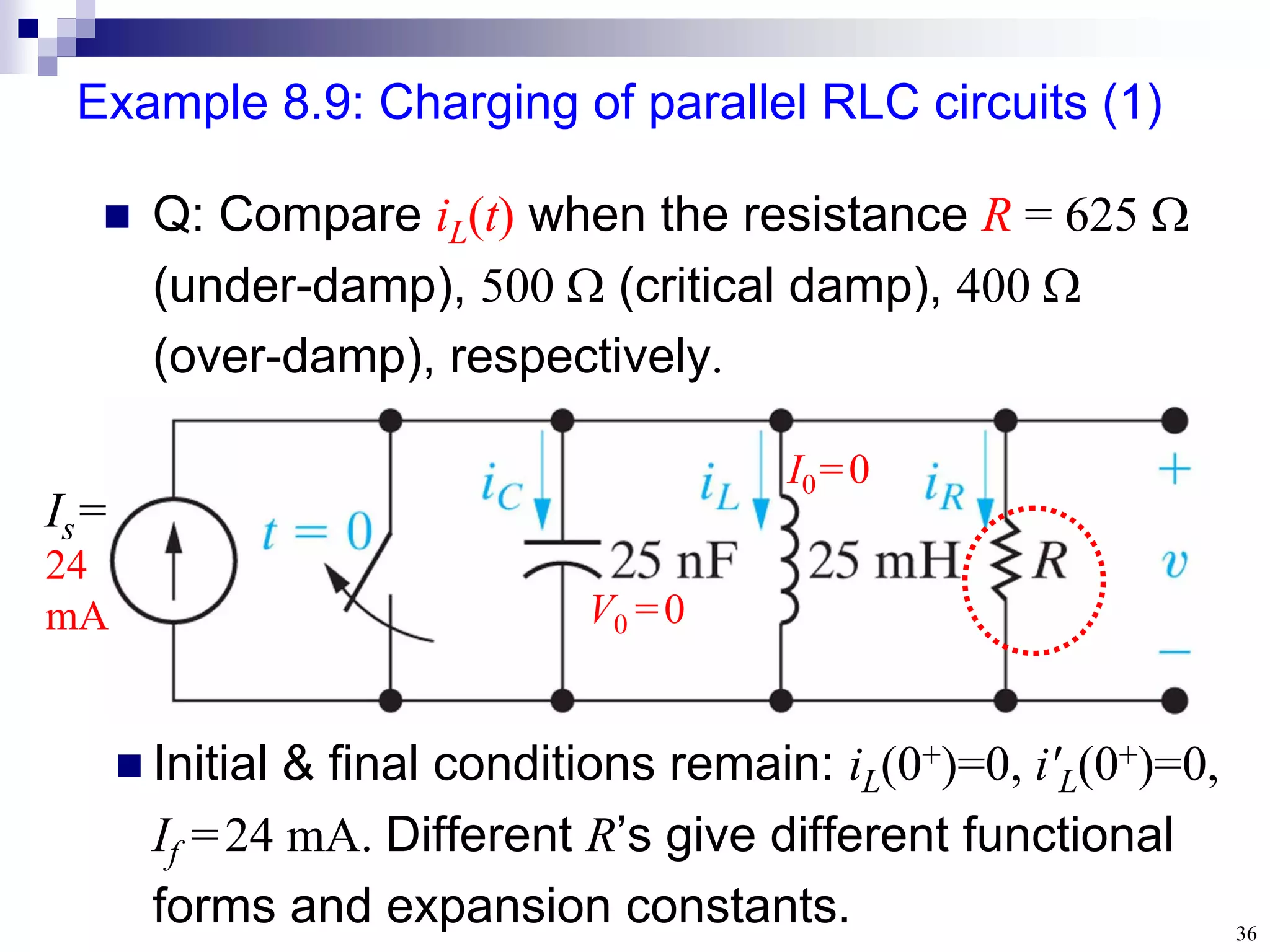
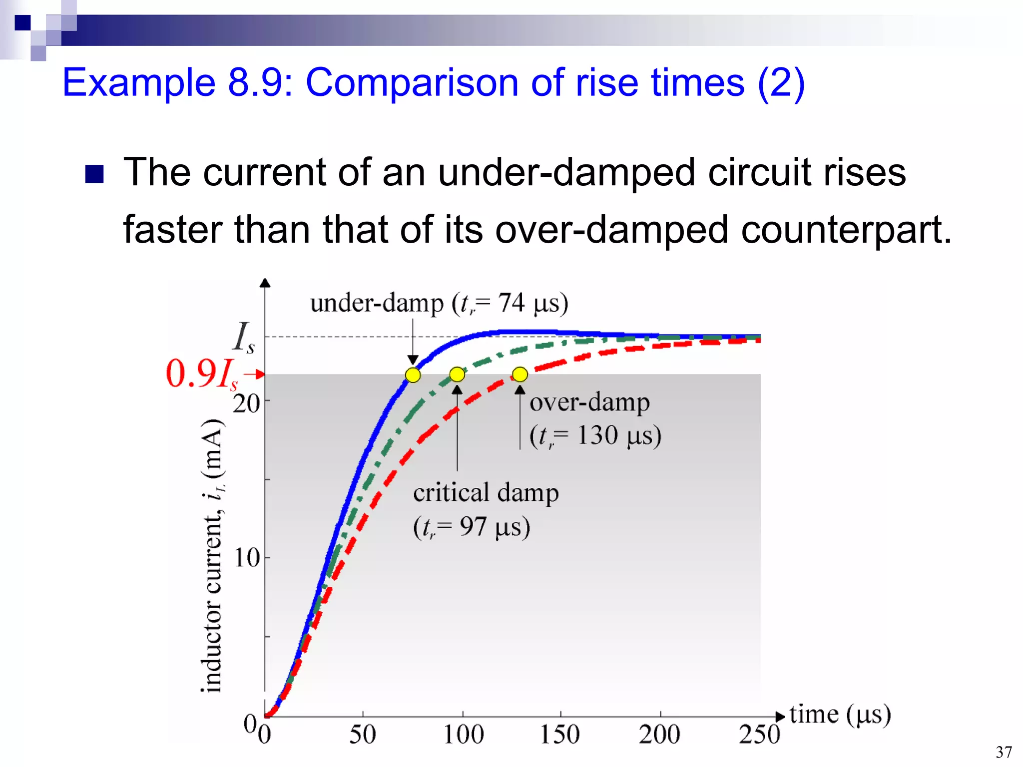
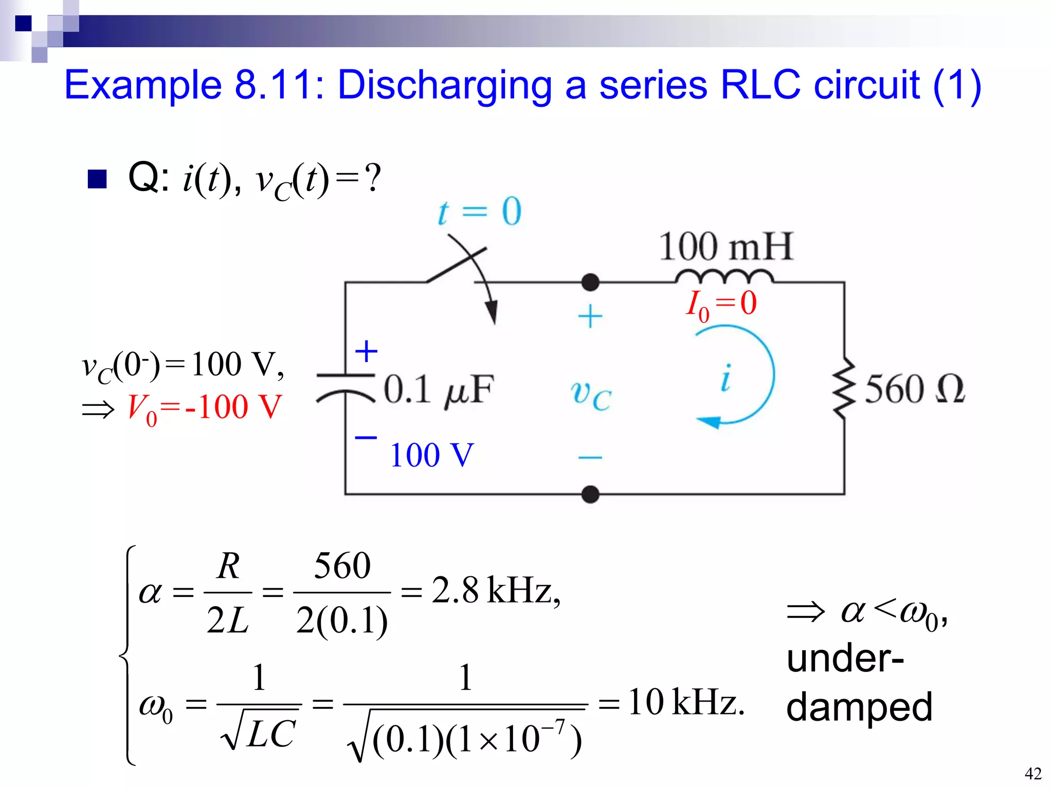
Example 8.9: Charging of parallel RLC circuits (1)
 Q: Compare iL(t) when the resistance R = 625 
(under-damp), 500  (critical damp), 400 
(over-damp), respectively.
Is=
24
mA
 Initial & final conditions remain: iL(0+)=0, i'L(0+)=0,
If =24 mA. Different R’s give different functional
forms and expansion constants.
V0 =0
I0=0

37. 37
Example 8.9: Comparison of rise times (2)
 The current of an under-damped circuit rises
faster than that of its over-damped counterpart.

38. 38
Section 8.4
The Natural and Step
Response of a Series RLC
Circuit
1. Modifications of time constant, neper
frequency

39. 39
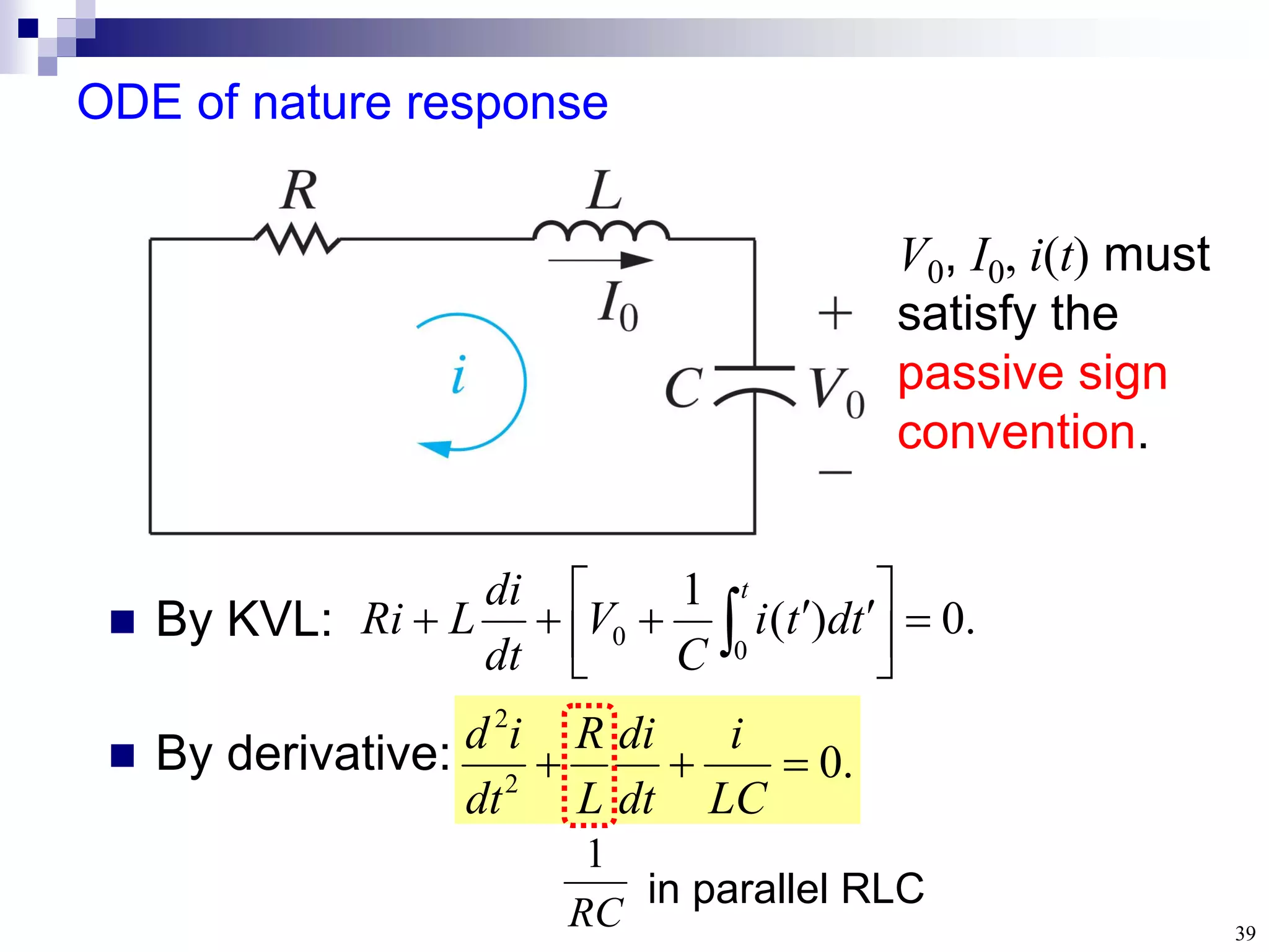
ODE of nature response
.
0
)
(
1
0
0 





 



 
t
t
d
t
i
C
V
dt
di
L
Ri
.
0
2
2



LC
i
dt
di
L
R
dt
i
d
RC
1
in parallel RLC
 By KVL:
 By derivative:
V0, I0, i(t) must
satisfy the
passive sign
convention.

40. 40
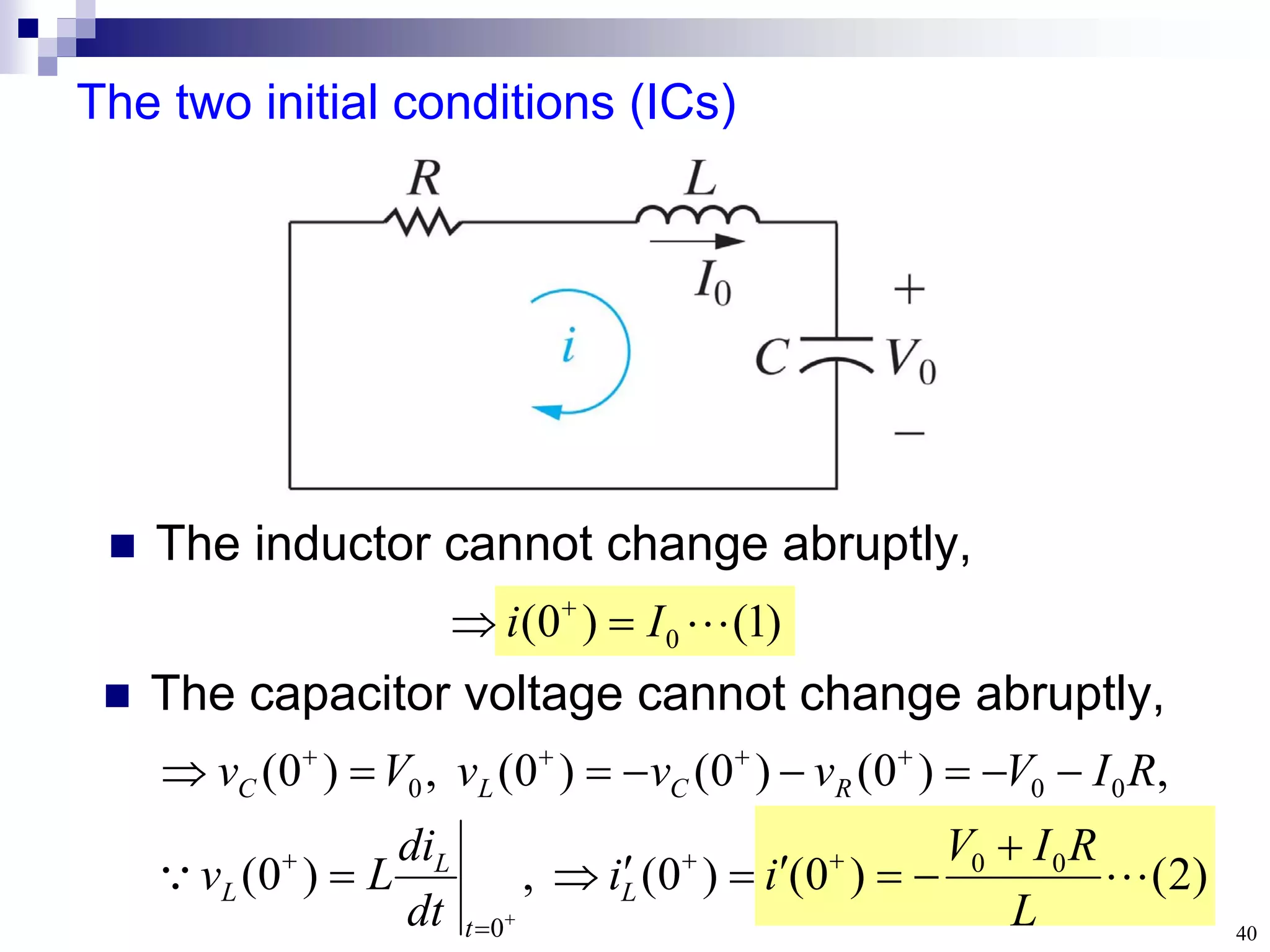
The two initial conditions (ICs)
 The inductor cannot change abruptly,
)
2
(
)
0
(
)
0
(
,
)
0
(
,
)
0
(
)
0
(
)
0
(
,
)
0
(
0
0
0
0
0
0


L
R
I
V
i
i
dt
di
L
v
R
I
V
v
v
v
V
v
L
t
L
L
R
C
L
C

























)
1
(
)
0
( 0 
I
i 
 
 The capacitor voltage cannot change abruptly,

41. 41
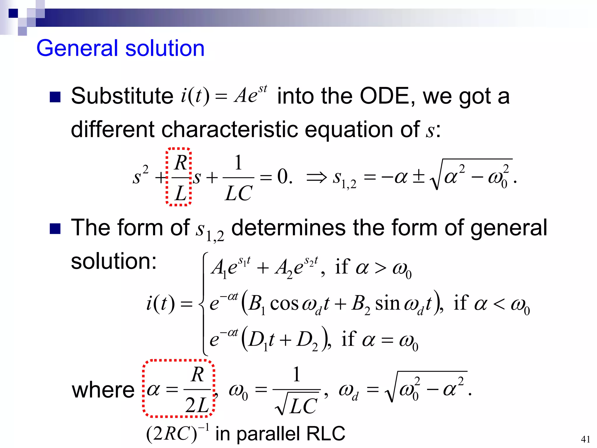
General solution
.
0
1
2



LC
s
L
R
s
 Substitute into the ODE, we got a
different characteristic equation of s:
st
Ae
t
i 
)
(
 
 














0
2
1
0
2
1
0
2
1
if
,
if
,
sin
cos
if
,
)
(
2
1










D
t
D
e
t
B
t
B
e
e
A
e
A
t
i
t
d
d
t
t
s
t
s
 The form of s1,2 determines the form of general
solution:
.
2
0
2
2
,
1 

 



 s
.
,
1
,
2
2
2
0
0 



 


 d
LC
L
R
where
1
)
2
( 
RC in parallel RLC

42. 42
Example 8.11: Discharging a series RLC circuit (1)
vC(0-)=100 V,
 V0=-100 V
I0 =0















kHz.
10
)
10
1
)(
1
.
0
(
1
1
,
kHz
8
.
2
)
1
.
0
(
2
560
2
7
0
LC
L
R

  <0,
under-
damped
 Q: i(t), vC(t)=?
+
 100 V

43. 43
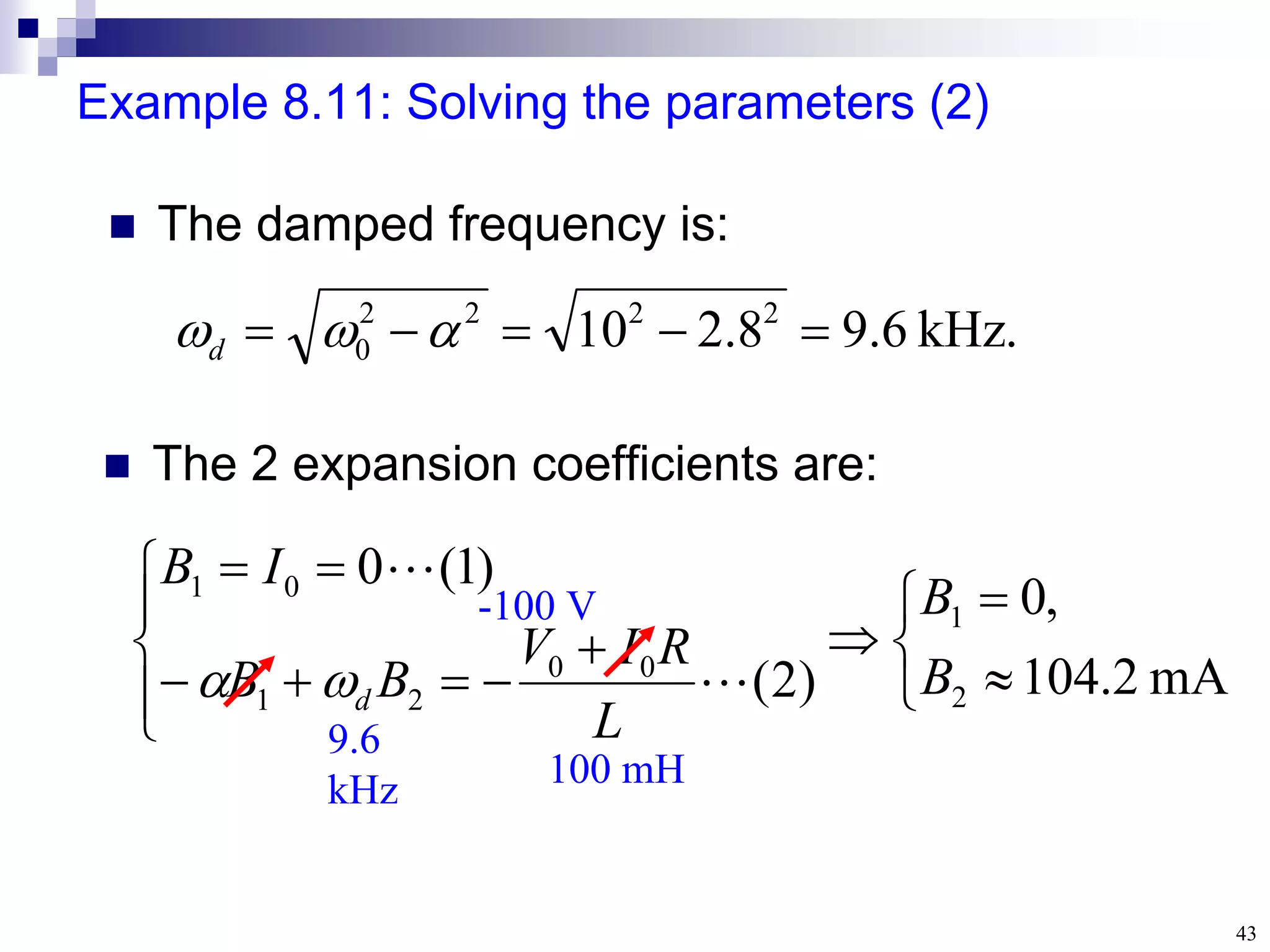
Example 8.11: Solving the parameters (2)
.
kHz
6
.
9
8
.
2
10 2
2
2
2
0 



 

d
 The damped frequency is:
 The 2 expansion coefficients are:


















mA
2
.
104
,
0
)
2
(
)
1
(
0
2
1
0
0
2
1
0
1
B
B
L
R
I
V
B
B
I
B
d 



9.6
kHz 100 mH
-100 V

44. 44
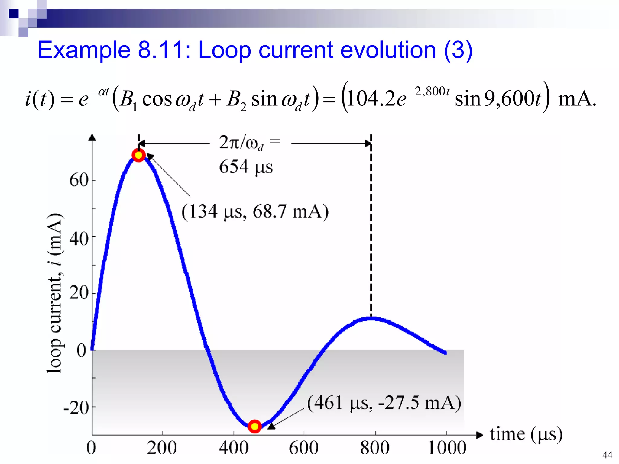
Example 8.11: Loop current evolution (3)
    .
mA
600
,
9
sin
2
.
104
sin
cos
)
( 800
,
2
2
1 t
e
t
B
t
B
e
t
i t
d
d
t 



 



45. 45
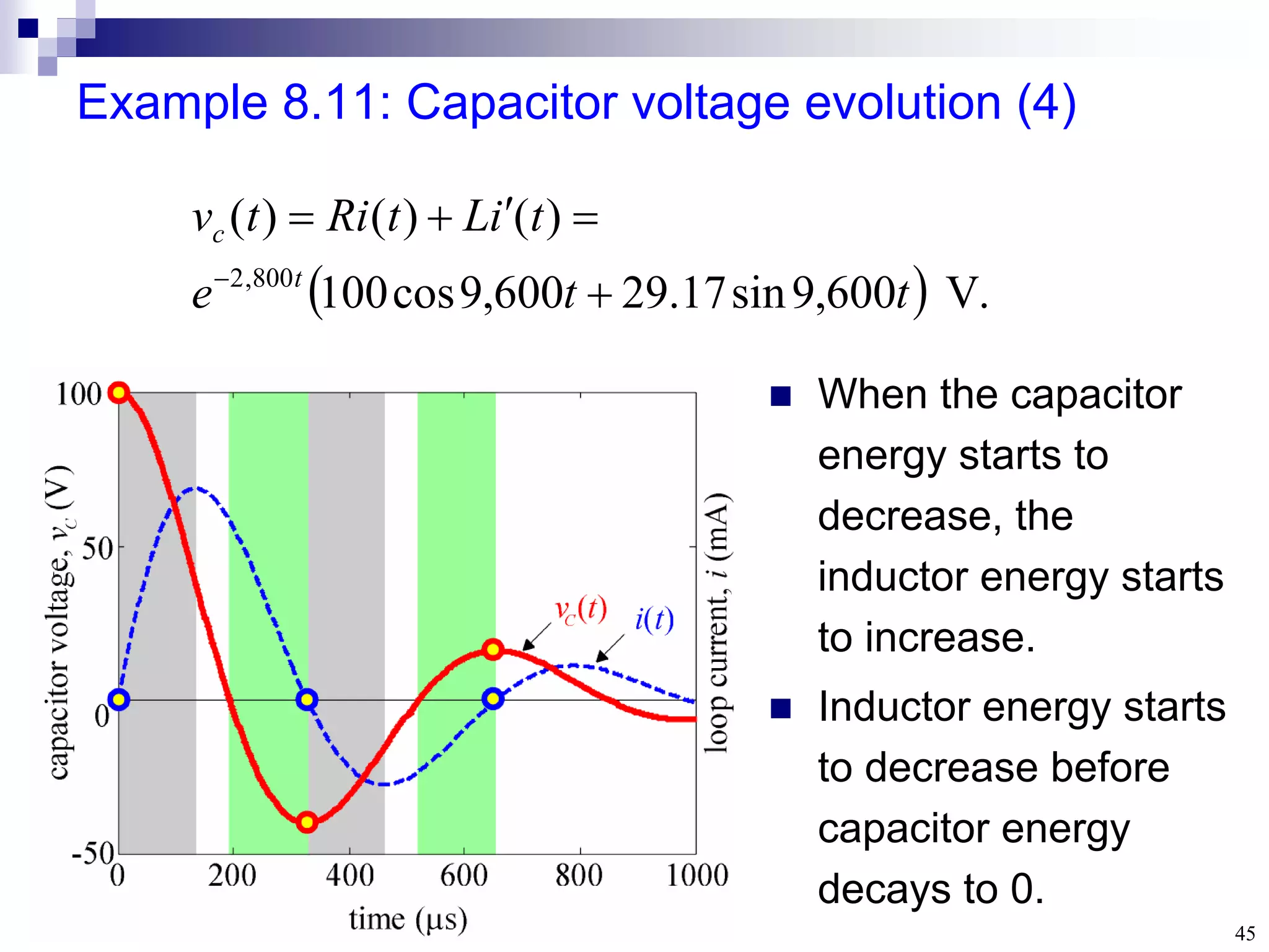
Example 8.11: Capacitor voltage evolution (4)
  .
V
600
,
9
sin
17
.
29
600
,
9
cos
100
)
(
)
(
)
(
800
,
2
t
t
e
t
i
L
t
Ri
t
v
t
c






 When the capacitor
energy starts to
decrease, the
inductor energy starts
to increase.
 Inductor energy starts
to decrease before
capacitor energy
decays to 0.

46. 46
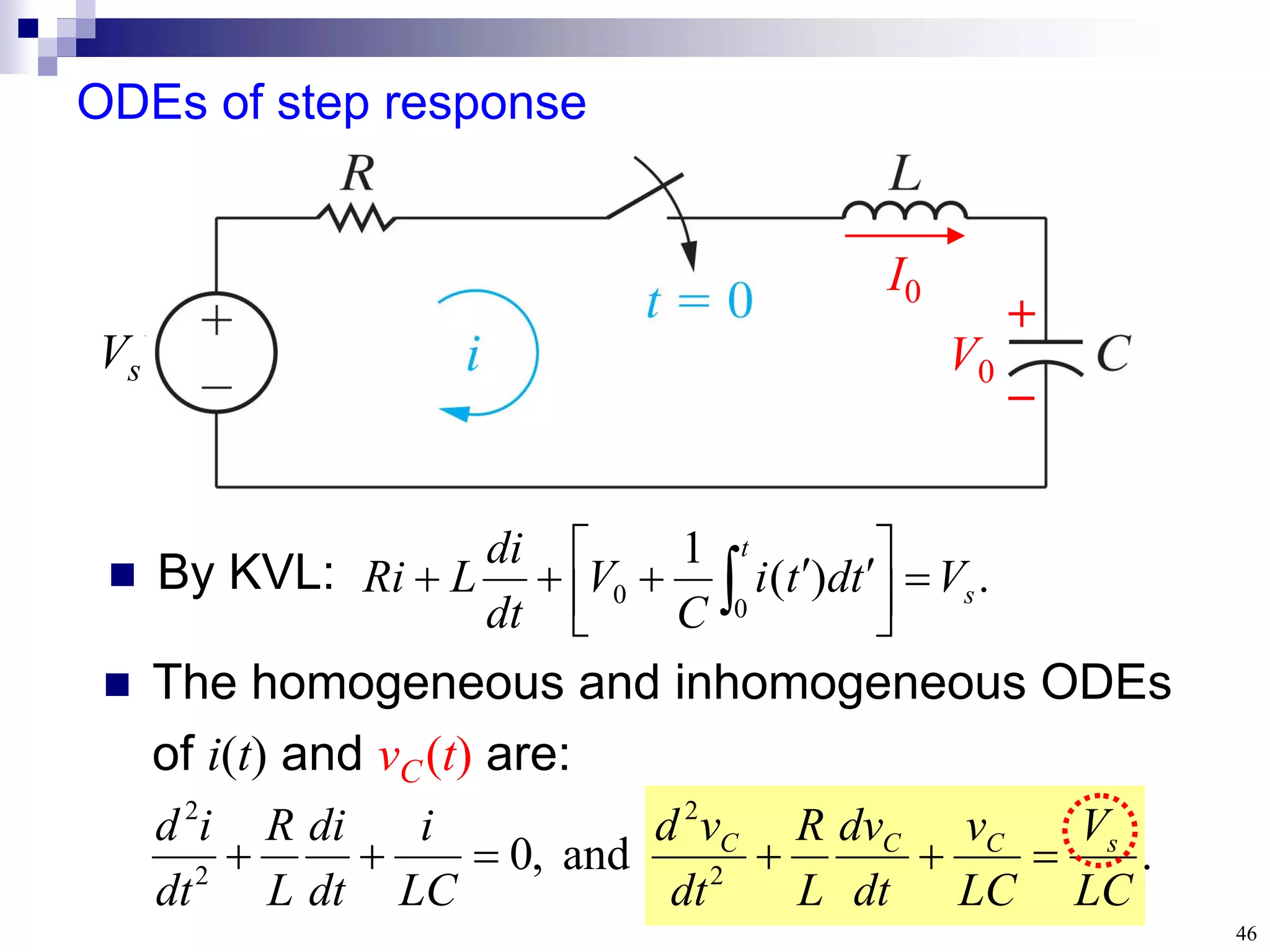
ODEs of step response
 By KVL:
 The homogeneous and inhomogeneous ODEs
of i(t) and vC(t) are:
V0
I0
Vs
+

.
)
(
1
0
0 s
t
V
t
d
t
i
C
V
dt
di
L
Ri 





 



 
.
and
,
0 2
2
2
2
LC
V
LC
v
dt
dv
L
R
dt
v
d
LC
i
dt
di
L
R
dt
i
d s
C
C
C







47. 47
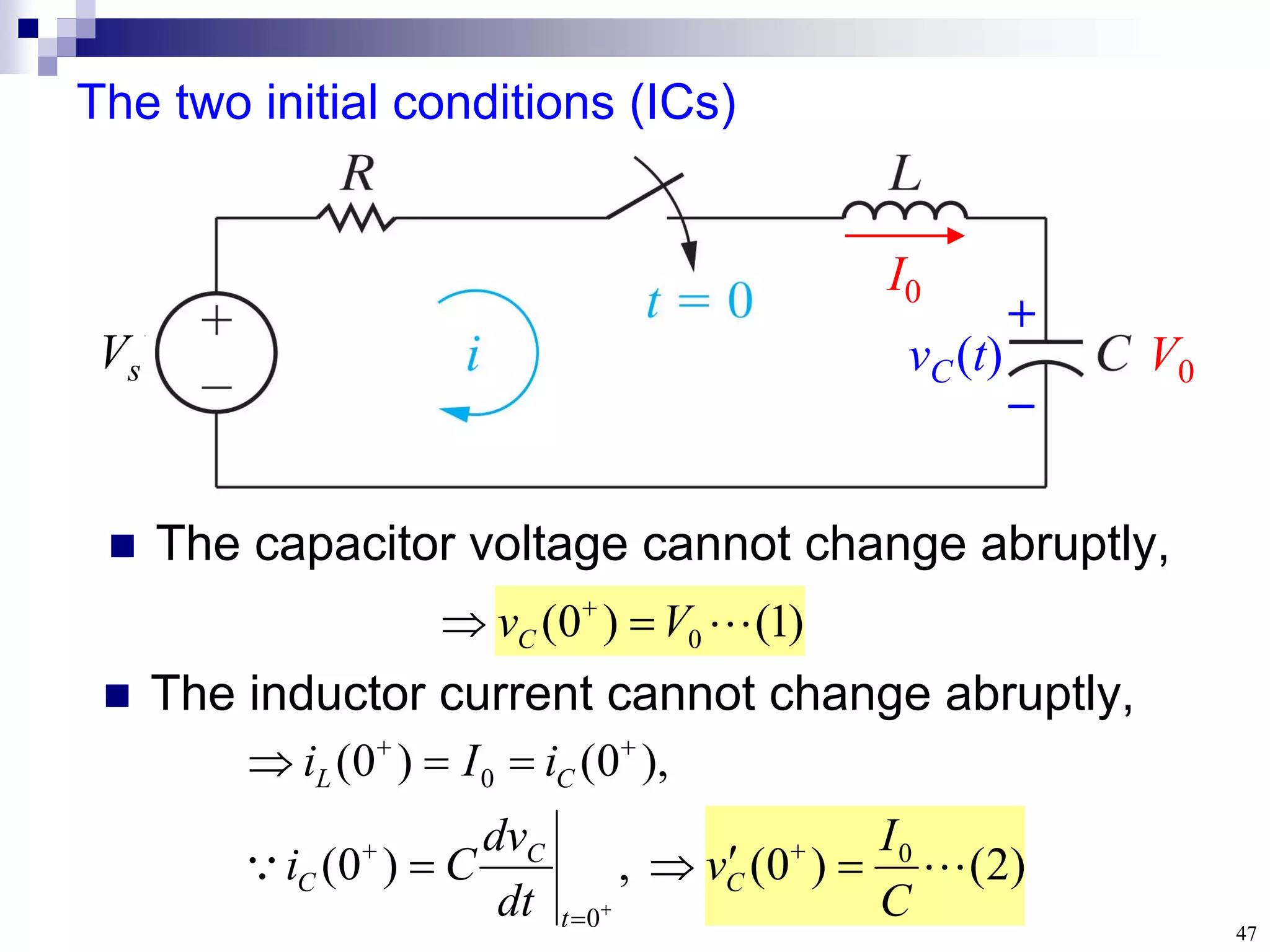
The two initial conditions (ICs)
 The capacitor voltage cannot change abruptly,
)
2
(
)
0
(
,
)
0
(
),
0
(
)
0
(
0
0
0


C
I
v
dt
dv
C
i
i
I
i
C
t
C
C
C
L













)
1
(
)
0
( 0 
V
vC 
 
 The inductor current cannot change abruptly,
V0
I0
Vs
+

vC(t)

48. 48
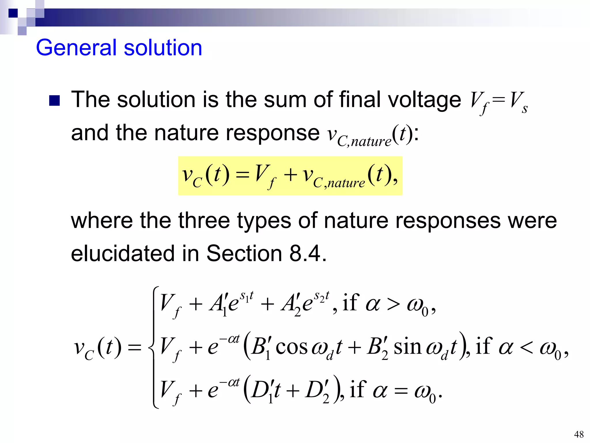
General solution
where the three types of nature responses were
elucidated in Section 8.4.
 The solution is the sum of final voltage Vf =Vs
and the nature response vC,nature(t):
),
(
)
( , t
v
V
t
v nature
C
f
C 

 
 

























.
if
,
,
if
,
sin
cos
,
if
,
)
(
0
2
1
0
2
1
0
2
1
2
1










D
t
D
e
V
t
B
t
B
e
V
e
A
e
A
V
t
v
t
f
d
d
t
f
t
s
t
s
f
C

49. 49
Key points
 What do the response curves of over-, under-,
and critically-damped circuits look like? How to
choose R, L, C values to achieve fast switching
or to prevent overshooting damage?
 What are the initial conditions in an RLC circuit?
How to use them to determine the expansion
coefficients of the complete solution?
 Comparisons between: (1) natural & step
responses, (2) parallel, series, or general RLC.