Chapter 5:Risk and Return

Find out more at www.kawsarbd1.weebly.com Last saved and edited by Md.Kawsar Siddiqui113
Principles of Managerial Finance Solution
Lawrence J. Gitman
CHAPTER 5
Risk and Return
INSTRUCTOR’S RESOURCES
Overview
This chapter focuses on the fundamentals of the risk and return relationship of assets and their valuation. For the
single asset held in isolation, risk is measured with the probability distribution and its associated statistics: the
mean, the standard deviation, and the coefficient of variation. The concept of diversification is examined by
measuring the risk of a portfolio of assets that are perfectly positively correlated, perfectly negatively correlated,
and those that are uncorrelated. Next, the chapter looks at international diversification and its effect on risk. The
Capital Asset Pricing Model (CAPM) is then presented as a valuation tool for securities and as a general
explanation of the risk-return trade-off involved in all types of financial transactions.
PMF DISK
This chapter's topics are not covered on the PMF Tutor or PMF Problem-Solver.
PMF Templates
Spreadsheet templates are provided for the following problems:
Problem Topic
Self-Test 1 Portfolio analysis
Self-Test 2 Beta and CAPM
Problem 5-7 Coefficient of variation
Problem 5-26 Security market line, SML

Chapter 5 Risk and Return
Study Guide
The following Study Guide examples are suggested for classroom presentation:
Example Topic
4 Risk attitudes
6 Graphic determination of beta
12 Impact of market changes on return

ANSWERS TO REVIEW QUESTIONS
5-1 Risk is defined as the chance of financial loss, as measured by the variability of expected returns associated
with a given asset. A decision maker should evaluate an investment by measuring the chance of loss, or
risk, and comparing the expected risk to the expected return. Some assets are considered risk-free; the
most common examples are U. S. Treasury issues.
5-2 The return on an investment (total gain or loss) is the change in value plus any cash distributions over a
defined time period. It is expressed as a percent of the beginning-of-the-period investment. The formula
is:
[ ]Return =
(ending value - initial value) + cash distribution
initial value
Realized return requires the asset to be purchased and sold during the time periods the return is measured.
Unrealized return is the return that could have been realized if the asset had been purchased and sold
during the time period the return was measured.
5-3 a. The risk-averse financial manager requires an increase in return for a given increase in risk.
b. The risk-indifferent manager requires no change in return for an increase in risk.
c. The risk-seeking manager accepts a decrease in return for a given increase in risk.
Most financial managers are risk-averse.
5-4 Sensitivity analysis evaluates asset risk by using more than one possible set of returns to obtain a sense of
the variability of outcomes. The range is found by subtracting the pessimistic outcome from the optimistic
outcome. The larger the range, the more variability of risk associated with the asset.
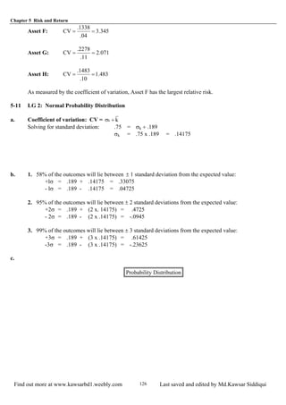
5-5 The decision maker can get an estimate of project risk by viewing a plot of the probability distribution,
which relates probabilities to expected returns and shows the degree of dispersion of returns. The more
spread out the distribution, the greater the variability or risk associated with the return stream.
5-6 The standard deviation of a distribution of asset returns is an absolute measure of dispersion of risk about
the mean or expected value. A higher standard deviation indicates a greater project risk. With a larger
standard deviation, the distribution is more dispersed and the outcomes have a higher variability, resulting
in higher risk.
5-7 The coefficient of variation is another indicator of asset risk, measuring relative dispersion. It is calculated
by dividing the standard deviation by the expected value. The coefficient of variation may be a better basis
than the standard deviation for comparing risk of assets with differing expected returns.
5-8 An efficient portfolio is one that maximizes return for a given risk level or minimizes risk for a given level
of return. Return of a portfolio is the weighted average of returns on the individual component assets:

∑=
×=
n
1j
jjp kˆwkˆ
Where n = number of assets, wj = weight of individual assets, and = expectedjkˆ
Returns.
The standard deviation of a portfolio is not the weighted average of component standard deviations; the
risk of the portfolio as measured by the standard deviation will be smaller. It is calculated by applying the
standard deviation formula to the portfolio assets:
σkp
i
i
n
k k
n
=
−
−=
∑
( )
( )
2
1 1
5-9 The correlation between asset returns is important when evaluating the effect of a new asset on the
portfolio's overall risk. Returns on different assets moving in the same direction are positively correlated,
while those moving in opposite directions are negatively correlated. Assets with high positive correlation
increase the variability of portfolio returns; assets with high negative correlation reduce the variability of
portfolio returns. When negatively correlated assets are brought together through diversification, the
variability of the expected return from the resulting combination can be less than the variability or risk of
the individual assets. When one asset has high returns, the other's returns are low and vice versa.
Therefore, the result of diversification is to reduce risk by providing a pattern of stable returns.
Diversification of risk in the asset selection process allows the investor to reduce overall risk by combining
negatively correlated assets so that the risk of the portfolio is less than the risk of the individual assets in it.
Even if assets are not negatively correlated, the lower the positive correlation between them, the lower the
resulting risks.
5-10 The inclusion of foreign assets in a domestic company's portfolio reduces risk for two reasons. When
returns from foreign-currency-denominated assets are translated into dollars, the correlation of returns of
the portfolio's assets is reduced. Also, if the foreign assets are in countries that are less sensitive to the
U.S. business cycle, the portfolio's response to market movements is reduced.
When the dollar appreciates relative to other currencies, the dollar value of a foreign-currency-
denominated portfolio declines and results in lower returns in dollar terms. If this appreciation is due to
better performance of the U.S. economy, foreign-currency-denominated portfolios generally have lower
returns in local currency as well, further contributing to reduced returns.
Political risks result from possible actions by the host government that are harmful to foreign investors or
possible political instability that could endanger foreign assets. This form of risk is particularly high in
developing countries. Companies diversifying internationally may have assets seized or the return of
profits blocked.
5-11 The total risk of a security is the combination of nondiversifiable risk and diversifiable risk. Diversifiable
risk refers to the portion of an asset's risk attributable to firm-specific, random events (strikes, litigation,
loss of key contracts, etc.) that can be eliminated by diversification. Nondiversifiable risk is attributable to
market factors affecting all firms (war, inflation, political events, etc.). Some argue that nondiversifiable
risk is the only relevant risk because diversifiable risk can be eliminated by creating a portfolio of assets
which are not perfectly positively correlated.
5-12 Beta measures nondiversifiable risk. It is an index of the degree of movement of an asset's return in
response to a change in the market return. The beta coefficient for an asset can be found by plotting the

asset's historical returns relative to the returns for the market. By using statistical techniques, the
"characteristic line" is fit to the data points. The slope of this line is beta. Beta coefficients for actively
traded stocks are published in Value Line Investment Survey and in brokerage reports. The beta of a
portfolio is calculated by finding the weighted average of the betas of the individual component assets.
5-13 The equation for the Capital Asset Pricing Model is: kj = RF+[bj x (km - RF)],
Where:
kj = the required (or expected) return on asset j.
RF = the rate of return required on a risk-free security (a U.S. Treasury bill)
bj = the beta coefficient or index of nondiversifiable (relevant) risk for asset j
km = the required return on the market portfolio of assets (the market return)
The security market line (SML) is a graphical presentation of the relationship between the amount of
systematic risk associated with an asset and the required return. Systematic risk is measured by beta and is
on the horizontal axis while the required return is on the vertical axis.
5-14 a. If there is an increase in inflationary expectations, the security market line will show a parallel shift
upward in an amount equal to the expected increase in inflation. The required return for a given level
of risk will also rise.
b. The slope of the SML (the beta coefficient) will be less steep if investors become less risk-averse, and
a lower level of return will be required for each level of risk.
5-15 The CAPM provides financial managers with a link between risk and return. Because it was developed to
explain the behavior of securities prices in efficient markets and uses historical data to estimate required
returns, it may not reflect future variability of returns. While studies have supported the CAPM when
applied in active securities markets, it has not been found to be generally applicable to real corporate
assets. However, the CAPM can be used as a conceptual framework to evaluate the relationship between
risk and return.

SOLUTIONS TO PROBLEMS
5-1 LG 1: Rate of Return:
1t
t1tt
t
P
)CPP(
k
−
− +−
=
a.
Investment X: Return %50.12
000,20$
)500,1$000,20$000,21($
=
+−
=
Investment Y: Return %36.12
000,55$
)800,6$000,55$000,55($
=
+−
=
b. Investment X should be selected because it has a higher rate of return for the same level of risk.
5-2 LG 1: Return Calculations:
1t
t1tt
t
P
)CPP(
k
−
− +−
=
Investment Calculation kt (%)
A ($1,100 - $800 - $100) ÷ $800 25.00
B ($118,000 - $120,000 + $15,000) ÷ $120,000 10.83
C ($48,000 - $45,000 + $7,000) ÷ $45,000 22.22
D ($500 - $600 + $80) ÷ $600 -3.33
E ($12,400 - $12,500 + $1,500) ÷ $12,500 11.20
5-3 LG 1: Risk Preferences
a. The risk-indifferent manager would accept Investments X and Y because these have higher returns than the
12% required return and the risk doesn’t matter.
b. The risk-averse manager would accept Investment X because it provides the highest return and has the
lowest amount of risk. Investment X offers an increase in return for taking on more risk than what the firm
currently earns.
c. The risk-seeking manager would accept Investments Y and Z because he or she is willing to take greater
risk without an increase in return.
d. Traditionally, financial managers are risk-averse and would choose Investment X, since it provides the
required increase in return for an increase in risk.
5-4 LG 2: Risk Analysis
a. Expansion Range
A 24% - 16% = 8%
B 30% - 10% = 20%
b. Project A is less risky, since the range of outcomes for A is smaller than the range for Project B.

c. Since the most likely return for both projects is 20% and the initial investments are equal, the answer
depends on your risk preference.
d. The answer is no longer clear, since it now involves a risk-return trade-off. Project B has a slightly higher
return but more risk, while A has both lower return and lower risk.
5-5 LG 2: Risk and Probability
a. Camera Range
R 30% - 20% = 10%
S 35% - 15% = 20%
b. Possible Probability Expected Return Weighted
Outcomes Pri ki Value (%)
(ki x Pri)
Camera R Pessimistic 0.25 20 5.00
Most likely 0.50 25 12.50
Optimistic 0.25 30 7.50
1.00 Expected Return 25.00
Camera S Pessimistic 0.20 15 3.00
Most likely 0.55 25 13.75
Optimistic 0.25 35 8.75
1.00 Expected Return 25.50
c. Camera S is considered more risky than Camera R because it has a much broader range of outcomes. The
risk-return trade-off is present because Camera S is more risky and also provides a higher return than
Camera R.

5-6 LG 2: Bar Charts and Risk
a.
Bar Chart-Line J
0
0.1
0.2
0.3
0.4
0.5
0.6
0.75 1.25 8.5 14.7Expected Return (%) 5 16.25
Probability
Bar Chart-Line K
0
0.1
0.2
0.3
0.4
0.5
0.6
1 2. 155 8 13.5
Expected Return (%)
Probability
b. Weighted
Market Probability Expected Return Value
Acceptance Pri ki (ki x Pri)
Line J Very Poor 0.05 .0075 .000375
Poor 0.15 .0125 .001875
Average 0.60 .0850 .051000
Good 0.15 .1475 .022125
Excellent 0.05 .1625 .008125
1.00 Expected Return .083500

Line K Very Poor 0.05 .010 .000500
Poor 0.15 .025 .003750
Average 0.60 .080 .048000
Good 0.15 .135 .020250
Excellent 0.05 .150 .007500
1.00 Expected Return .080000
c. Line K appears less risky due to a slightly tighter distribution than line J, indicating a lower range of
outcomes.
5-7 LG 2: Coefficient of Variation:
k
CV
kσ
=
a. A 3500.
%20
%7
CVA ==
B 4318.
%22
%5.9
CVB ==
C 3158.
%19
%6
CVC ==
D 3438.
%16
%5.5
CVD ==
b. Asset C has the lowest coefficient of variation and is the least risky relative to the other choices.
5-8 LG 2: Standard Deviation versus Coefficient of Variation as Measures of Risk
a. Project A is least risky based on range with a value of .04.
b. Project A is least risky based on standard deviation with a value of .029. Standard deviation is not the
appropriate measure of risk since the projects have different returns.
c. A 2417.
12.
029.
CVA ==
B 2560.
125.
032.
CVB ==
C 2692.
13.
035.
CVC ==
D .2344
128.
030.
CVD ==
In this case project A is the best alternative since it provides the least amount of risk for each percent of
return earned. Coefficient of variation is probably the best measure in this instance since it provides a
standardized method of measuring the risk/return trade-off for investments with differing returns.

5-9 LG 2: Assessing Return and Risk
a. Project 257
1. Range: 1.00 - (-.10) = 1.10
2. Expected return: ir
n
1i
i Pkk ∑=
×=
Rate of Return Probability Weighted Value Expected Return
ki Pri ki x Pri ir
n
1i
i Pkk ∑=
×=
-.10 .01 -.001
.10 .04 .004
.20 .05 .010
.30 .10 .030
.40 .15 .060
.45 .30 .135
.50 .15 .075
.60 .10 .060
.70 .05 .035
.80 .04 .032
1.00 .01 .010
1.00 .450
3. Standard Deviation: ∑=
−=
n
1i
i )kk(σ 2
x Pri
2
Pri )kk( i − 2
x Priki k kki − )kk( i −
-.10 .450 -.550 .3025 .01 .003025
.10 .450 -.350 .1225 .04 .004900
.20 .450 -.250 .0625 .05 .003125
.30 .450 -.150 .0225 .10 .002250
.40 .450 -.050 .0025 .15 .000375
.45 .450 .000 .0000 .30 .000000
.50 .450 .050 .0025 .15 .000375
.60 .450 .150 .0225 .10 .002250
.70 .450 .250 .0625 .05 .003125
.80 .450 .350 .1225 .04 .004900
1.00 .450 .550 .3025 .01 .003025.
.027350
σProject 257 = .027350 = .165378
4. 3675.
450.
165378.
CV ==
Project 432
1. Range: .50 - .10 = .40
2. Expected return: ir
n
1i
i Pkk ∑=
×=

ki Pri ki x Pri ir
n
1i
i Pkk ∑=
×=
.10 .05 .0050
.15 .10 .0150
.20 .10 .0200
.25 .15 .0375
.30 .20 .0600
.35 .15 .0525
.40 .10 .0400
.45 .10 .0450
.50 .05 .0250
1.00 .300
3. Standard Deviation: ∑=
−=σ
n
1i
i )kk( 2
x Pri
ki k kki − )kk( i − 2
Pri )kk( i − 2
x Pri
.10 .300 -.20 .0400 .05 .002000
.15 .300 -.15 .0225 .10 .002250
.20 .300 -.10 .0100 .10 .001000
.25 .300 -.05 .0025 .15 .000375
.30 .300 .00 .0000 .20 .000000
.35 .300 .05 .0025 .15 .000375
.40 .300 .10 .0100 .10 .001000
.45 .300 .15 .0225 .10 .002250
.50 .300 .20 .0400 .05 .002000
.011250
σProject 432 = .011250 = .106066
4. 3536.
300.
106066.
CV ==
b. Bar Charts
Project 257
Probability

c.
Summa
ry Statistics
Project 257 Project 432
0
0.05
0.1
0.15
0.2
0.25
0.3
-10% 30% 40% 60% 70% 80% 100%
Rate of Return
Project 432
10% 20% 45% 50%
Range 1.100 .400
Expected
Return ( k ) 0.450 .300
Standard
Deviation ( ) 0.165 .106kσ
Coefficient of
Variation (CV) 0.3675 .3536
0
0.05
0.15
0.2
0.25
0.3
20% 25% 35% 40% 45% 50%
Probability
0.1
10% 15% 30%
Since Projects 257 and 432 have differing expected values, the coefficient of variation
should be the criterion by which the risk of the asset is judged. Since Project 432 has
a smaller CV, it is the opportunity with lower risk.
Rate of Return
5-10 LG 2: Integrative–Expected Return, Standard Deviation, and Coefficient of Variation
a. Expected return: ∑=
×=
n
1i
iri Pkk
ki Pri ki x Pri ir
n
1i
i Pkk ∑=
×=
Asset F .40 .10 .04
.10 .20 .02
.00 .40 .00
-.05 .20 -.01
-.10 .10 -.01
.04

Asset G .35 .40 .14
.10 .30 .03
-.20 .30 -.06
.11
Asset H .40 .10 .04
.20 .20 .04
.10 .40 .04
.00 .20 .00
-.20 .10 -.02
.10
Asset G provides the largest expected return.
b. Standard Deviation: ∑=
−=σ
n
1i
ik )kk( 2
x Pri
)kk( i − )kk( i − 2
P σri
2
σk
Asset F .40 - .04 = .36 .1296 .10 .01296
.10 - .04 = .06 .0036 .20 .00072
.00 - .04 = -.04 .0016 .40 .00064
-.05 - .04 = -.09 .0081 .20 .00162
-.10 - .04 = -.14 .0196 .10 .00196
.01790 .1338
)kk( i − )kk( i − 2
P σri
2
σk
Asset G .35 - .11 = .24 .0576 .40 .02304
.10 - .11 = -.01 .0001 .30 .00003
-.20 - .11 = -.31 .0961 .30 .02883
.05190 .2278
Asset H .40 - .10 = .30 .0900 .10 .009
.20 - .10 = .10 .0100 .20 .002
.10 - .10 = .00 .0000 -.40 .000
.00 - .10 = -.10 .0100 .20 .002
-.20 - .10 = -.30 .0900 .10 .009
.022 .1483
Based on standard deviation, Asset G appears to have the greatest risk, but it must be measured against its
expected return with the statistical measure coefficient of variation, since the three assets have differing
expected values. An incorrect conclusion about the risk of the assets could be drawn using only the
standard deviation.
c.
valueexpected
)(deviationstandard
=VariationoftCoefficien
σ

Asset F: 345.3
04.
1338.
CV ==
Asset G: 071.2
11.
2278.
CV ==
Asset H: 483.1
10.
1483.
CV ==
As measured by the coefficient of variation, Asset F has the largest relative risk.
5-11 LG 2: Normal Probability Distribution
a. Coefficient of variation: CV = kk ÷σ
Solving for standard deviation: .75 = σk ÷ .189
σk = .75 x .189 = .14175
b. 1. 58% of the outcomes will lie between ± 1 standard deviation from the expected value:
+lσ = .189 + .14175 = .33075
- lσ = .189 - .14175 = .04725
2. 95% of the outcomes will lie between ± 2 standard deviations from the expected value:
+2σ = .189 + (2 x. 14175) = .4725
- 2σ = .189 - (2 x .14175) = -.0945
3. 99% of the outcomes will lie between ± 3 standard deviations from the expected value:
+3σ = .189 + (3 x .14175) = .61425
-3σ = .189 - (3 x .14175) = -.23625
c.
Probability Distribution

0
10
20
30
40
50
60
-0.236 -0.094 0.047 0.331 0.473 0.6140.189Return
Probability
5-12 LG 3: Portfolio Return and Standard Deviation
a. Expected Portfolio Return for Each Year: kp = (wL x kL) + (wM x kM)
Expected
Asset L Asset M Portfolio Return
Year (wL x kL) + (wM x kM) kp
2004 (14% x.40 = 5.6%) + (20% x .60 = 12.0%) = 17.6%
2005 (14% x.40 = 5.6%) + (18% x .60 = 10.8%) = 16.4%
2006 (16% x.40 = 6.4%) + (16% x .60 = 9.6%) = 16.0%
2007 (17% x.40 = 6.8%) + (14% x .60 = 8.4%) = 15.2%
2008 (17% x.40 = 6.8%) + (12% x .60 = 7.2%) = 14.0%
2009 (19% x.40 = 7.6%) + (10% x .60 = 6.0%) = 13.6%
b. Portfolio Return:
n
kw
k
n
1j
jj
p
∑=
×
=
%5.15467.15
6
6.130.142.150.164.166.17
kp ==
+++++
=
c. Standard Deviation: σkp
i
i
n
k k
n
=
−
−=
∑
( )
( )
2
1 1

16
%)5.15%6.13(%)5.15%0.14(%)5.15%2.15(
%)5.15%0.16(%)5.15%4.16(%)5.15%6.17(
222
222
kp
−
⎥
⎥
⎦
⎤
⎢
⎢
⎣
⎡
−+−+−+
−+−+−
=σ
5
%)9.1(%)5.1(%)3.0(
%)5.0(%)9(.%)1.2(
222
222
kp
⎥
⎥
⎦
⎤
⎢
⎢
⎣
⎡
−+−+−+
++
=σ
5
%)61.3%25.2%09.0%25.0%81.0%41.4(
kp
+++++
=σ
51129.1284.2
5
42.11
kp ===σ
d. The assets are negatively correlated.
e. Combining these two negatively correlated assets reduces overall portfolio risk.
5-13 LG 3: Portfolio Analysis
a. Expected portfolio return:
Alternative 1: 100% Asset F
%5.17
4
%19%18%17%16
kp =
+++
=
Alternative 2: 50% Asset F + 50% Asset G
Asset F Asset G Portfolio Return
Year (wF x kF) + (wG x kG) kp
2001 (16% x .50 = 8.0%) + (17% x .50 = 8.5%) = 16.5%
2002 (17% x .50 = 8.5%) + (16% x .50 = 8.0%) = 16.5%
2003 (18% x .50 = 9.0%) + (15% x .50 = 7.5%) = 16.5%
2004 (19% x .50 = 9.5%) + (14% x .50 = 7.0%) = 16.5%
%5.16
4
66
kp ==
Alternative 3: 50% Asset F + 50% Asset H
Asset F Asset H Portfolio Return
Year (wF x kF) + (wH x kH) kp
2001 (16% x .50 = 8.0%) + (14% x .50 = 7.0%) 15.0%
2002 (17% x .50 = 8.5%) + (15% x .50 = 7.5%) 16.0%
2003 (18% x .50 = 9.0%) + (16% x .50 = 8.0%) 17.0%
2004 (19% x .50 = 9.5%) + (17% x .50 = 8.5%) 18.0%

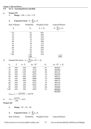
%5.16
4
66
kp ==
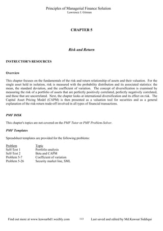
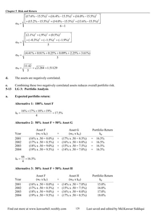
b. Standard Deviation: σkp
i
i
n
k k
n
=
−
−=
∑
( )
( )
2
1 1
(1)
[ ]
14
%)5.17%0.19(%)5.17%0.18(%)5.17%0.17(%)5.17%0.16( 2222
F
−
−+−+−+−
=σ
[ ]
3
%)5.1(%)5.0(%)5.0(%)-1.5( 2222
F
++−+
=σ
3
%)25.2%25.0%25.0%25.2(
F
+++
=σ
291.1667.1
3
5
F ===σ
(2)
[ ]
14
%)5.16%5.16(%)5.16%5.16(%)5.16%5.16(%)5.16%5.16( 2222
FG
−
−+−+−+−
=σ
[ ]
3
)0()0()0()0( 2222
FG
+++
=σ
0FG =σ
(3)
[ ]σFH =
− + − + − + −
−
( . . ( . . ( . . ( . .150% 165%) 160% 165%) 17 0% 165%) 180% 165%)
4 1
2 2 2 2
[ ]
3
%)5.1(%)5.0(%)5.0(%)5.1( 2222
FH
++−+−
=σ
[ ]
3
)25.225.25.25.2(
FH
+++
=σ

291.1667.1
3
5
FH ===σ
c. Coefficient of variation: CV = kk ÷σ
0738.
%5.17
291.1
CVF ==
0
%5.16
0
CVFG ==
0782.
%5.16
291.1
CVFH ==
d. Summary:
kp: Expected Value
of Portfolio σkp CVp
Alternative 1 (F) 17.5% 1.291 .0738
Alternative 2 (FG) 16.5% -0- .0
Alternative 3 (FH) 16.5% 1.291 .0782
Since the assets have different expected returns, the coefficient of variation should be used to determine
the best portfolio. Alternative 3, with positively correlated assets, has the highest coefficient of variation
and therefore is the riskiest. Alternative 2 is the best choice; it is perfectly negatively correlated and
therefore has the lowest coefficient of variation.
5-14 LG 4: Correlation, Risk, and Return
a. 1. Range of expected return: between 8% and 13%
2. Range of the risk: between 5% and 10%
b. 1. Range of expected return: between 8% and 13%
2. Range of the risk: 0 < risk < 10%
c. 1. Range of expected return: between 8% and 13%
2. Range of the risk: 0 < risk < 10%
5-15 LG 1, 4: International Investment Returns
a. Returnpesos = %73.2020732.
500,20
250,4
500,20
500,20750,24
===
−
b. 84.225,2$shares000,122584.2$
21.9
50.20
dollarperPesos
pesosinPrice
pricePurchase =×==

69.512,2$shares000,151269.2$
85.9
75.24
dollarperPesos
pesosinPrice
pricealesS =×==
c. Returnpesos = %89.1212887.
84.225,2
85.286
84.225,2
84.225,269.512,2
===
−
d. The two returns differ due to the change in the exchange rate between the peso and the dollar. The peso
had depreciation (and thus the dollar appreciated) between the purchase date and the sale date, causing a
decrease in total return. The answer in part c is the more important of the two returns for Joe. An investor
in foreign securities will carry exchange-rate risk.
5-16 LG 5: Total, Nondiversifiable, and Diversifiable Risk
a. and b.
c. Only nondiversifiable risk
is relevant because, as
shown by the graph, diversifiable risk can be virtually eliminated through holding a portfolio of at least 20
securities which are not positively correlated. David Talbot's portfolio, assuming diversifiable risk could
no longer be reduced by additions to the portfolio, has 6.47% relevant risk.
0
2
4
6
8
10
12
14
16
0 5 10 15 20
Number of Securities
DiversifiableNondiversifiable
Portfolio
Risk
(σkp)
(%)
5-17 LG 5: Graphic Derivation of Beta

a. Derivation of Beta
b. To estimate
beta, the "rise over
run" method can be
used:
Beta =
Rise
Run
=
∆
∆
Y
X
Taking the
points shown on the
graph:
75.
4
3
48
912
==
−
−
X
Y
=ABeta =
∆
∆
33.1
3
4
1013
2226
X
Y
=BBeta ==
−
−
=
∆
∆
-12
-8
-4
0
4
8
12
16
20
24
28
32
-16 -12 -8 -4 0 4 8 12 16
Asset B
Asset A
Market Return
Asset Return %
b = slope = 1.33
b = slope = .75
A financial calculator with statistical functions can be used to perform linear regression analysis. The beta
(slope) of line A is .79; of line B, 1.379.
c. With a higher beta of 1.33, Asset B is more risky. Its return will move 1.33 times for each one point the
market moves. Asset A’s return will move at a lower rate, as indicated by its beta coefficient of .75.
5-18 LG 5: Interpreting Beta
Effect of change in market return on asset with beta of 1.20:
a. 1.20 x (15%) = 18.0% increase
b. 1.20 x (-8%) = 9.6% decrease
c. 1.20 x (0%) = no change
d. The asset is more risky than the market portfolio, which has a beta of 1. The higher beta makes the
return move more than the market.
5-19 LG 5: Betas
a. and b.
Increase in Expected Impact Decrease in Impact on
Asset Beta Market Return on Asset Return Market Return Asset Return
A 0.50 .10 .05 -.10 -.05
B 1.60 .10 .16 -.10 -.16
C - 0.20 .10 -.02 -.10 .02
D 0.90 .10 .09 -.10 -.09
c. Asset B should be chosen because it will have the highest increase in return.
d. Asset C would be the appropriate choice because it is a defensive asset, moving in opposition to the
market. In an economic downturn, Asset C's return is increasing.
5-20 LG 5: Betas and Risk Rankings
a. Stock Beta
Most risky B 1.40
A 0.80

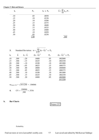
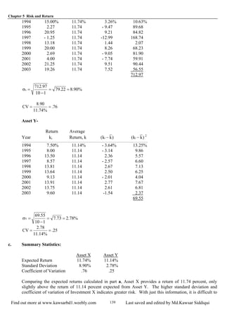
Least risky C -0.30
b. and c. Increase in Expected Impact Decrease in Impact on
Asset Beta Market Return on Asset Return Market Return Asset Return
A 0.80 .12 .096 -.05 -.04
B 1.40 .12 .168 -.05 -.07
C - 0.30 .12 -.036 -.05 .015
d. In a declining market, an investor would choose the defensive stock, stock C. While the market declines,
the return on C increases.
e. In a rising market, an investor would choose stock B, the aggressive stock. As the market rises one point,
stock B rises 1.40 points.
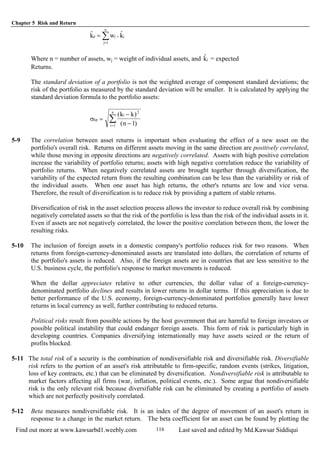
5-21 LG 5: Portfolio Betas: bp = ∑=
×
n
1j
jj bw
a.
Portfolio A Portfolio B
Asset Beta wA wA x bA wB wB x bB
1 1.30 .10 .130 .30 .39
2 0.70 .30 .210 .10 .07
3 1.25 .10 .125 .20 .25
4 1.10 .10 .110 .20 .22
5 .90 .40 .360 .20 .18
bA = .935 bB = 1.11
b. Portfolio A is slightly less risky than the market (average risk), while Portfolio B is more risky than the
market. Portfolio B's return will move more than Portfolio A’s for a given increase or decrease in market
return. Portfolio B is the more risky.
5-22 LG 6: Capital Asset Pricing Model (CAPM): kj = RF + [bj x (km - RF)]
Case kj = RF + [bj x (km - RF)]
A 8.9% = 5% + [1.30 x (8% - 5%)]
B 12.5% = 8% + [0.90 x (13% - 8%)]
C 8.4% = 9% + [- 0.20 x (12% - 9%)]
D 15.0% = 10% + [1.00 x (15% - 10%)]
E 8.4% = 6% + [0.60 x (10% - 6%)]
5-23 LG 6: Beta Coefficients and the Capital Asset Pricing Model
To solve this problem you must take the CAPM and solve for beta. The resulting model is:
Fm
F
Rk
Rk
Beta
−
−
=
a. 4545.
%11
%5
%5%16
%5%10
Beta ==
−
−
=
b. 9091.
%11
%10
%5%16
%5%15
Beta ==
−
−
=

c. 1818.1
%11
%13
%5%16
%5%18
Beta ==
−
−
=
d. 3636.1
%11
%15
%5%16
%5%20
Beta ==
−
−
=
e. If Katherine is willing to take a maximum of average risk then she will be able to have an expected return
of only 16%. (k = 5% + 1.0(16% - 5%) = 16 %.)
5-24 LG 6: Manipulating CAPM: kj = RF + [bj x (km - RF)]
a. kj = 8% + [0.90 x (12% - 8%)]
kj = 11.6%
b. 15% = RF + [1.25 x (14% - RF)]
RF = 10%
c. 16% = 9% + [1.10 x (km - 9%)]
km = 15.36%
d. 15% = 10% + [bj x (12.5% - 10%)
bj = 2
5-25 LG 1, 3, 5, 6: Portfolio Return and Beta
a. bp = (.20)(.80)+(.35)(.95)+(.30)(1.50)+(.15)(1.25) = .16+.3325+.45+.1875=1.13
b. %8
000,20$
600,1$
000,20$
600,1$)000,20$000,20($
kA ==
+−
=
%86.6
000,35$
400,2$
000,35$
400,1$)000,35$000,36($
kB ==
+−
=
%15
000,30$
500,4$
000,30$
0)000,30$500,34($
kC ==
+−
=
%5.12
000,15$
875,1$
000,15$
375$)000,15$500,16($
kD ==
+−
=
c. %375.10
000,100$
375,10$
000,100$
375,3$)000,100$000,107($
kP ==
+−
=
d. kA = 4% + [0.80 x (10% - 4%)] = 8.8%
kB = 4% + [0.95 x (10% - 4%)] = 9.7%
kC = 4% + [1.50 x (10% - 4%)] = 13.0%
kD = 4% + [1.25 x (10% - 4%)] = 11.5%

e. Of the four investments, only C had an actual return which exceeded the CAPM expected return (15%
versus 13%). The underperformance could be due to any unsystematic factor which would have caused
the firm not do as well as expected. Another possibility is that the firm's characteristics may have changed
such that the beta at the time of the purchase overstated the true value of beta that existed during that year.
A third explanation is that beta, as a single measure, may not capture all of the systematic factors that
cause the expected return. In other words, there is error in the beta estimate.
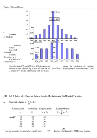
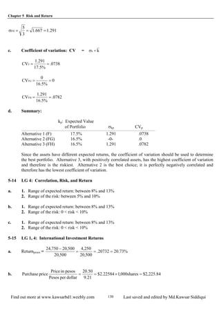
5-26 LG 6: Security Market Line, SML
a., b., and d.
Security Market Line
0
2
4
6
8
10
12
14
16
0 0.2 0.4 0.6 0.8 1 1.2 1.4
S
Ris
A
K
B
Risk premiumMarket Risk
Required Rate
of Return %
Nondiversifiable Risk (Beta)
c. kj RF + [bj x (km - RF)]
Asset A
kj = .09 + [0.80 x (.13 -.09)]
kj = .122
Asset B
kj = .09 + [1.30 x (.13 -.09)]
kj = .142
d. Asset A has a smaller required return than Asset B because it is less risky, based on the beta of 0.80 for
Asset A versus 1.30 for Asset B. The market risk premium for Asset A is 3.2% (12.2% - 9%), which is
lower than Asset B's (14.2% - 9% = 5.2%).

Find out m w.kawsarbd1.weebly.com Last saved and edited by Md.Kawsar Siddiqui136
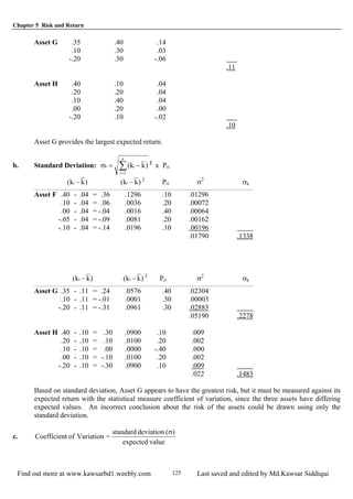
5-27 LG 6: Shifts in the Security Market Line
a., b., c., d.
Security Market Lines
b. kj = RF + [bj x (km - RF)]
ore at ww
kA = 8% + [1.1 x (12% -
8%)]
kA =
8%
+ 4.4%
kA =
12.4%
c. kA = 6% + [1.1 x (10% - 6%)]
kA = 6% + 4.4%0
2
4
8
10
12
14
16
18
20
0 0.2 0.4 0.6 0.8 1 1.2 1.4 1.6 1.8 2
Asset A
Asset A
SMLd
SMLa
SMLc
Required
Return
(%)
6
kA = 10.4%
d. kA = 8% + [1.1 x (13% - 8%)]
kA = 8% + 5.5%
kA = 13.5%
e. 1. A decrease in inflationary expectations reduces the required return as shown in the parallel downward
shift of the SML.
2. Increased risk aversion results in a steeper slope, since a higher return would be required for each level
of risk as measured by beta.
5-28 LG 5, 6: Integrative-Risk, Return, and CAPM
a. Project kj = RF + [bj x (km - RF)]
A kj = 9% + [1.5 x (14% - 9%)] = 16.5%
B kj = 9% + [.75 x (14% - 9%)] = 12.75%
C kj = 9% + [2.0 x (14% - 9%)] = 19.0%
D kj = 9% + [ 0 x (14% - 9%)] = 9.0%
E kj = 9% + [(-.5) x (14% - 9%)] = 6.5%
b. and d.
Security Market Line
SMLb
SMLd
Required
Rate of
Return
(%)

c. Project A is 150% as responsive
as the market.
Project B is 75% as responsive as
the market.
Project C is twice as responsive
as the market.
Project D is unaffected by market
movement.
Project E is only half as
responsive as the market, but
moves in the opposite direction as
the market.
d. See graph for new SML.
kA = 9% + [1.5 x (12% - 9%)]
kB = 9% + [.75 x (12% - 9%)]
kC = 9% + [2.0 x (12% - 9%)]
kD = 9% + [0 x (12% -
9%)] = 9.00%
kE = 9% + [-.5 x (12% - 9%)]
0
2
4
6
8
10
12
14
16
18
20
-0.5 0 0.5 1 1.5 2
e. The steeper slope of SMLb indicates a higher risk premium than SMLd for these market conditions. When
investor risk aversion declines, investors require lower returns for any given risk level (beta).

Chapter 5 Case
Analyzing Risk and Return on Chargers Products' Investments
This case requires students to review and apply the concept of the risk-return trade-off by analyzing two possible
asset investments using standard deviation, coefficient of variation, and CAPM.
a.
Expected rate of return:
1t
t1tt
t
P
)CPP(
k
−
− +−
=
Asset X:
Cash Ending Beginning Gain/ Annual Rate
Year Flow (Ct) Value (Pt) Value (Pt-1) Loss of Return
1994 $1,000 $22,000 $20,000 $2,000 15.00%
1995 1,500 21,000 22,000 - 1,000 2.27
1996 1,400 24,000 21,000 3,000 20.95
1997 1,700 22,000 24,000 - 2,000 - 1.25
1998 1,900 23,000 22,000 1,000 13.18
1999 1,600 26,000 23,000 3,000 20.00
2000 1,700 25,000 26,000 - 1,000 2.69
2001 2,000 24,000 25,000 - 1,000 4.00
2002 2,100 27,000 24,000 3,000 21.25
2003 2,200 30,000 27,000 3,000 19.26
Average expected return for Asset X = 11.74%
Asset Y:
Cash Ending Beginning Gain/ Annual Rate
Year Flow (Ct) Value (Pt) Value (Pt-1) Loss of Return
1994 $1,500 $20,000 $20,000 $0 7.50%
1995 1,600 20,000 20,000 0 8.00
1996 1,700 21,000 20,000 1,000 13.50
1997 1,800 21,000 21,000 0 8.57
1998 1,900 22,000 21,000 1,000 13.81
1999 2,000 23,000 22,000 1,000 13.64
2000 2,100 23,000 23,000 0 9.13
2001 2,200 24,000 23,000 1,000 13.91
2002 2,300 25,000 24,000 1,000 13.75
2003 2,400 25,000 25,000 0 9.60
Average expected return for Asset Y = 11.14%
b.
σk = ∑=
−÷−
n
1i
2
i )1n()kk(
Asset X:
Return Average
Year ki Return, k )kk( i − )kk( i − 2

1994 15.00% 11.74% 3.26% 10.63%
1995 2.27 11.74 - 9.47 89.68
1996 20.95 11.74 9.21 84.82
1997 - 1.25 11.74 -12.99 168.74
1998 13.18 11.74 1.44 2.07
1999 20.00 11.74 8.26 68.23
2000 2.69 11.74 - 9.05 81.90
2001 4.00 11.74 - 7.74 59.91
2002 21.25 11.74 9.51 90.44
2003 19.26 11.74 7.52 56.55
712.97
%90.822.79
110
97.712
x ==
−
=σ
76.
%74.11
90.8
CV ==
Asset Y-
Return Average
Year ki Return, k )kk( i − )kk( i − 2
1994 7.50% 11.14% - 3.64% 13.25%
1995 8.00 11.14 - 3.14 9.86
1996 13.50 11.14 2.36 5.57
1997 8.57 11.14 - 2.57 6.60
1998 13.81 11.14 2.67 7.13
1999 13.64 11.14 2.50 6.25
2000 9.13 11.14 - 2.01 4.04
2001 13.91 11.14 2.77 7.67
2002 13.75 11.14 2.61 6.81
2003 9.60 11.14 -1.54 2.37
69.55
%78.273.7
110
55.69
Y ==
−
=σ
25.
%14.11
78.2
CV ==
c. Summary Statistics:
Asset X Asset Y
Expected Return 11.74% 11.14%
Standard Deviation 8.90% 2.78%
Coefficient of Variation .76 .25
Comparing the expected returns calculated in part a, Asset X provides a return of 11.74 percent, only
slightly above the return of 11.14 percent expected from Asset Y. The higher standard deviation and
coefficient of variation of Investment X indicates greater risk. With just this information, it is difficult to

determine whether the .60 percent difference in return is adequate compensation for the difference in risk.
Based on this information, however, Asset Y appears to be the better choice.
d. Using the capital asset pricing model, the required return on each asset is as follows:
Capital Asset Pricing Model: kj = RF + [bj x (km - RF)]
Asset RF + [bj x (km - RF)] = kj
X 7% + [1.6 x (10% - 7%)] = 11.8%
Y 7% + [1.1 x (10% - 7%)] = 10.3%
From the calculations in part a, the expected return for Asset X is 11.74%, compared to its required return
of 11.8%. On the other hand, Asset Y has an expected return of 11.14% and a required return of only
10.8%. This makes Asset Y the better choice.
e. In part c, we concluded that it would be difficult to make a choice between X and Y because the additional
return on X may or may not provide the needed compensation for the extra risk. In part d, by calculating a
required rate of return, it was easy to reject X and select Y. The required return on Asset X is 11.8%, but
its expected return (11.74%) is lower; therefore Asset X is unattractive. For Asset Y the reverse is true,
and it is a good investment vehicle.
Clearly, Charger Products is better off using the standard deviation and coefficient of variation, rather than
a strictly subjective approach, to assess investment risk. Beta and CAPM, however, provide a link
between risk and return. They quantify risk and convert it into a required return that can be compared to
the expected return to draw a definitive conclusion about investment acceptability. Contrasting the
conclusions in the responses to questions c and d above should clearly demonstrate why Junior is better off
using beta to assess risk.
f. (1) Increase in risk-free rate to 8 % and market return to 11 %:
X 8% + [1.6 x (11% - 8%)] = 12.8%
Y 8% + [1.1 x (11% - 8%)] = 11.3%
(2) Decrease in market return to 9 %:
X 7% + [1.6 x (9% - 7%)] = 10.2%
Y 7% + [1.1 x (9% -7%)] = 9.2%
In situation (1), the required return rises for both assets, and neither has an expected return above the firm's
required return.
With situation (2), the drop in market rate causes the required return to decrease so that the expected
returns of both assets are above the required return. However, Asset Y provides a larger return compared
to its required return (11.14 - 9.20 = 1.94), and it does so with less risk than Asset X.

Chapter 5:Risk and Return

More Related Content

What's hot

Similar to Chapter 5:Risk and Return

More from Inocentshuja Ahmad

Recently uploaded

Chapter 5:Risk and Return