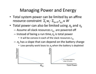
This document discusses resource management for computer operating systems. It argues that traditional OS architecture is outdated given changes in hardware and software. The authors propose an approach where the OS allocates resources like CPU cores, memory, and bandwidth to processes to optimize responsiveness based on penalty functions that model how run time affects user experience. The goal is to continuously minimize the total penalty by adjusting resource allocations over time as user needs and process requirements change.

1. Resource
Management
for
Computer
Opera3ng
Systems
Sarah
Bird
PhD
Candidate
Berkeley
EECS
Burton
Smith
Technical
Fellow
MicrosoB

2. OS
Architecture
Is
Ancient

3. Hardware
Has
Changed

4. SoBware
Has
Changed

5. A
Way
Forward
• Resources
should
be
allocated
to
processes
– Cores
of
various
types
– Memory
(working
sets)
– Bandwidths,
e.g.
to
shared
caches,
memory,
storage
and
interconnec3on
networks
• The
opera3ng
system
should:
– Op3mize
the
responsiveness
of
the
system
– Respond
to
changes
in
user
expecta3ons
– Respond
to
changes
in
process
requirements
– Maintain
resource,
power
and
energy
constraints
What
follows
is
a
scheme
to
realize
this
vision

6. Responsiveness
• Run
3mes
determine
process
responsiveness
– The
3me
from
a
mouse
click
to
its
result
– The
3me
from
a
service
request
to
its
response
– The
3me
from
job
launch
to
job
comple3on
– The
3me
to
execute
a
specified
amount
of
work
• The
rela3onship
is
usually
a
nonlinear
one
– Achievable
responses
may
be
needlessly
fast
– There
is
generally
a
threshold
of
acceptability
• Run
3me
depends
on
the
resources
– Some
resources
will
have
more
effect
than
others
– Effects
will
oBen
vary
with
computa3onal
phase

7. Penalty
Func3ons
• The
penalty
func.on
of
a
process
defines
how
run
3mes
translate
into
responsiveness
– Its
shape
expresses
the
nonlinearity
of
the
rela3onship
– The
shape
will
depend
on
the
applica3on
and
on
the
current
user
interface
state
(e.g.
minimized)
• We
let
the
total
penalty
be
the
instantaneous
sum
of
the
current
penal3es
of
the
running
processes
– Resources
determine
run
3mes
and
therefore
penal3es
• Assigning
resources
to
processes
to
minimize
the
total
penalty
maximizes
system
responsiveness

8. Typical
Penalty
Func3ons
Run
.me
Penalty
Deadline
Run
.me
Penalty

9. Adjus3ng
Penalty
Func3ons
• Penalty
func3ons
are
like
priori3es,
except:
– They
apply
to
processes,
not
kernel
threads
– They
are
explicit
convex
func3ons
of
the
run
3me
• The
opera3ng
system
can
adjust
their
slopes
– Up
or
down,
based
on
user
behavior
or
preference
– The
deadlines
can
probably
be
leB
alone
• The
total
penalty
is
easy
to
compute
– The
objec3ve
is
to
keep
minimizing
it

10. Run
Time
Func3ons
• Generally,
they
exhibit
“diminishing
returns”
as
resources
are
added
to
a
process
– That
is,
run
3mes
are
roughly
convex
func3ons
• They
vary
with
input
and
must
be
measured
– Some3mes
run
3me
increases
with
some
resource
– We
may
see
“plateaus”
or
various
types
of
“noise”
Run
3me
Memory
alloca3on

11. Resource
Alloca3on
As
Op3miza3on
Con3nuously
minimize
Σp∈P
πp(τp(rp,0,
…
rp,n-­‐1)
with
respect
to
the
resource
alloca3ons
rp,j
,
where
• P,
πp,
τp,
and
the
rp,j
are
all
3me-­‐varying;
• P
is
the
set
of
runnable
processes;
• rp,j
≥
0
is
the
alloca3on
of
resource
j
to
process
p;
• The
penalty
πp
depends
on
the
run
3me
τp;
• τp
depends
in
turn
on
the
allocated
resources
rp,j;
• Σp∈P
rp,j
=
Aj
,
the
available
quan3ty
of
resource
j.
– All
unused
(slack)
resources
are
allocated
to
process
0

12. The
Op3miza3on
Picture
Run3me1(r(0,1),
…,
r(n-­‐1,1))
Run3me1
Penalty1
Con3nuously
minimize
the
total
penalty
Run3me2
(r(0,2),
…,
r(n-­‐1,2))
Run3me2
Run3mei(r(0,i),
…,
r(n-­‐1,i))
Run3mei
Penalty2
Penaltyi
Subject
to
the
total
available
resources

13. Convexity
and
Concavity
• A
func3on
f
is
convex
if
for
all
x,
y
in
ℜn,
λ
in
ℜ,
and
0
≤
λ
≤
1,
f(λx
+
(1−λ)y)
≤
λf(x)
+
(1−λ)f(y)
– Chords
of
the
func3on’s
graph
must
lie
on
or
above
it
• A
func3on
f
is
concave
if
for
all
x,
y
in
ℜn,
λ
in
ℜ,
and
0
≤
λ
≤
1,
f(λx
+
(1−λ)y)
≥
λf(x)
+
(1−λ)f(y)
– Alterna3vely,
f
is
concave
if
and
only
if
–f
is
convex
• Affine
func3ons
Ax
+
b
are
both
convex
and
concave
• If
func3ons
fi
are
convex
so
is
their
sum
Σi
fi
• If
func3ons
fi
are
convex
so
is
their
maximum
maxi
fi
• If
f
is
both
convex
and
monotone
non-­‐decreasing
and
g
is
convex
then
h(x)
=
f(g(x))
is
convex
• If
f
is
convex,
so
is
the
set
Cα
=
{
x∈dom(f)
|
f(x)≤α
}
– Cα
is
called
the
α-­‐sublevel
set
of
f

14. Convex
Op3miza3on
• A
convex
op3miza3on
problem
has
the
form:
Minimize
f0(x1,
…
xm)
subject
to
fi(x1,
…
xm)
≤
0,
i
=
1,
…
k
where
the
func3ons
fi
:
Rm
→
R
are
all
convex
• Convex
op3miza3on
has
several
virtues
– It
guarantees
a
single
global
op3mal
value
– It
is
not
much
slower
than
linear
programming
• In
our
formula3on,
resource
management
is
a
convex
op3miza3on
problem

15. Managing
Power
and
Energy
• Total
system
power
can
be
limited
by
an
affine
resource
constraint
Σj
wj
·∙
Σp≠
0
rp,j
≤
W
• Total
power
can
also
be
limited
using
π0
and
τ0
– Assume
all
slack
resources
r0,j
are
powered
off
– Instead
of
being
a
run
3me,τ0
is
total
power
• It
will
be
convex
in
each
of
the
slack
resources
r0,j
– π0
has
a
slope
that
can
depend
on
the
bagery
charge
• Low-­‐penalty
work
loses
to
π0
when
the
bagery
is
depleted
Total
Power
Penalty
As
charge
depletes,
slope
increases
a0,r
Total
Power

16. Modeling
Run
Times
• Run
3me
measurements
can
be
used
to
construct
a
model,
yielding
several
advantages
– “Noise”
can
be
removed
while
building
the
model
– Interpola3on
among
measurements
is
avoided
– Rates
of
change
with
resources
are
computable
• We
have
constructed
several
types
of
model
– Linear
and
quadra3c
(rate)
models
–
Kernel
Canonical
Correla3on
Analysis
– Gene3cally
Programmed
Response
Surfaces
– Convex
non-­‐nega3ve
least
squares
models

17. Convex
Models
17
w:
learned
parameters
b:
bandwidth
alloca3ons
α:
bandwidth
amplifica3ons
m:
memory
alloca3ons
∑+=
ji ji
ji
bb
w
Tbw
,
,
0
*
),(τ
3
3
2
2
1
1
0),(
b
w
m
w
b
w
Tbw +++=τ
( )∑+=
i iii
i
mb
w
Tmbw
α
ατ 0),,,(

20. Modeling
Results
• Non-­‐nega3ve
least-­‐squares
applied
to
past
run
3me
data
learns
the
model
parameters
– Rows
of
the
QR
factoriza3on
are
updated
and
downdated
to
track
changes
in
process
behavior
– Columns
are
also
updated
and
downdated
to
remove
and
restore
infeasible
alloca3ons
• Our
convex
models
fit
the
data
quite
well
– They
work
even
beger
within
the
control
loop
– We
have
discovered
some
interes3ng
ar3facts

21. Nbodies
Frame
Time
0.01
0.1
0
500
1000
1500
2000
2500
3000
3500
Seconds
Memory
Pages
1
2
3
4
5
6
7
8
9
10
11
12
13
14
15
16

22. PACORA
• PACORA
stands
for
“Performance-­‐Aware
Convex
Op3miza3on
for
Resource
Alloca3on”
– See
our
paper
in
the
poster
session
of
HotPar
‘11
• It
manages
resource
alloca3on
policy
in
the
Berkeley
ParLab’s
Tessela3on
opera3ng
system
– One
of
us
(Bird)
is
currently
demonstra3ng
it
• Nearly
all
of
the
ideas
presented
here
are
being
prototyped
in
PACORA
and
Tessela3on
– Perhaps
they
may
be
valuable
elsewhere

23. PolicyService
Major
Change
Request
ACK/
NACK
App
Creation
and
Resizing
Requests
from Users
Admission
Control
Minor
Changes
ACK/NACK
App App App
All system
resources
App group
with fraction
of resources
App
Current
Application
Store
(Current Resources)
Global Policies /
User Policies and
Preferences
Offline Models
and Behavioral
Parameters
Build and
Refine
Resource
Value
Functions
App#1
App#2
App#3
User/System
Convex
Optimization
Set Penalty
Functions
Decision Validation
23
PACORA
in
Tessella3on
Resource
Allocations
Performance/
Energy Counters

24. Acknowledgements
• Stephen
Boyd
and
Lieven
Vandenberghe,
whose
book
taught
us
about
convex
op3miza3on
• Krste
Asanović,
David
Pagerson,
and
John
Kubiatowicz
at
Berkeley,
for
their
strong
support
• The
MicrosoB
Windows
developers,
for
giving
us
real
applica3ons
and
ways
to
measure
them
• Colleagues
at
the
UC
Berkeley
ParLab
and
at
MicrosoB
Research,
for
helping
us
tell
the
story

25. Thanks!
Any
ques3ons?