Download as PDF, PPTX


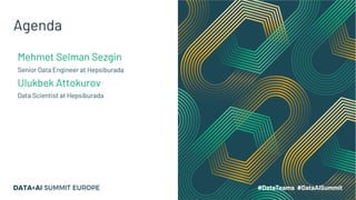
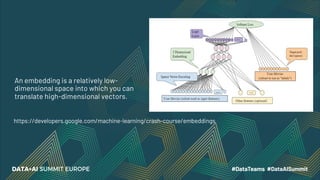
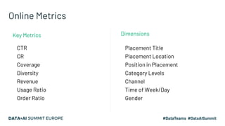
![Data Preparation
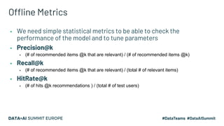
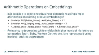
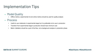
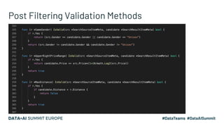
▪ Sentence
▪ Bag-of-Words
▪ “I am attending a conference”
▪ [“I”, “attending”, “conference”]
▪ User behavior (views, purchases etc.)
▪ Set of purchased items
▪ Orders: Keyboard, Computer, Mouse
▪ [“Keyboard”, “Computer”, “Mouse”]
Frequently Bought TogetherNLP](https://image.slidesharecdn.com/48attokurovsezgin-201124204022/85/Frequently-Bought-Together-Recommendations-Based-on-Embeddings-10-320.jpg)
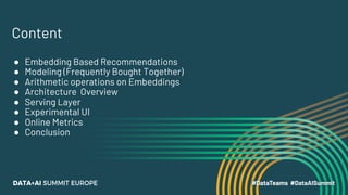
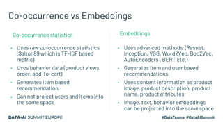
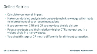
![Data Preparation - Context Separation
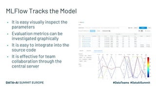
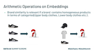
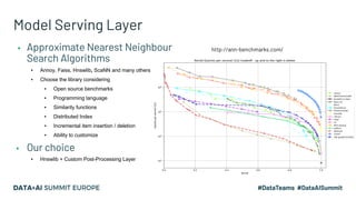
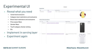
▪ Sequences may contain the products
from diverse categories
▪ [“Keyboard”, “Mouse”, “Shoes”, “Socks”]
▪ Sub-sequences may be created depending
on labels as category, brand etc.
▪ [“Keyboard”, “Mouse”] and [“Shoes”,Socks”]
Sub-sequenceSequence](https://image.slidesharecdn.com/48attokurovsezgin-201124204022/85/Frequently-Bought-Together-Recommendations-Based-on-Embeddings-11-320.jpg)

The document discusses an embedding-based recommendation system used to generate 'frequently bought together' suggestions at Hepsiburada, addressing challenges such as managing diverse product categories and customer behavior data. It details the technical foundation including the use of Word2Vec for data preparation, the architecture of the recommendation service, and various performance metrics for evaluating its effectiveness. Key takeaways emphasize the importance of embedding representations, careful parameter tuning, and the significance of online metrics for evaluating the recommendation system's impact.


![제 20회 보아즈(BOAZ) 빅데이터 컨퍼런스 - [데시벨] : 만월회를 위한 마케팅 데이터 분ᄉ...](https://cdn.slidesharecdn.com/ss_thumbnails/random-240811072343-5d8beb5d-thumbnail.jpg?width=640&height=640&fit=bounds)