Download to read offline


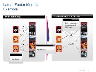
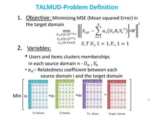

![How to win Netflix Prize with a few
lines of code:
movie_count = 17771
user_count = 2649430
model_left = Sequential()
model_left.add(Embedding(movie_count, 60, input_length=1))
model_right = Sequential()
model_right.add(Embedding(user_count, 20, input_length=1))
model = Sequential()
model.add(Merge([model_left, model_right], mode='concat'))
model.add(Flatten())
model.add(Dense(64))
model.add(Activation('sigmoid'))
model.add(Dense(64))
model.add(Activation('sigmoid'))
model.add(Dense(64))
model.add(Activation('sigmoid'))
model.add(Dense(1))
model.compile(loss='mean_squared_error', optimizer='adadelta')
model.fit([tr[:,0].reshape((L,1)), tr[:,1].reshape((L,1))], tr[:,2].reshape((L,1)), batch_size=24000,
nb_epoch=42, validation_data=([ ts[:,0].reshape((M,1)), ts[:,1].reshape((M,1))], ts[:,2].reshape((M,1))))](https://image.slidesharecdn.com/rokach-gomaxslides1-220424155654/85/Rokach-GomaxSlides-1-pptx-44-320.jpg)
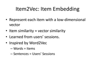
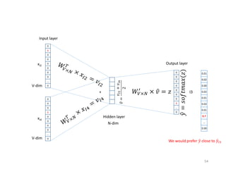

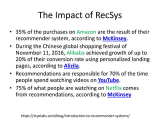
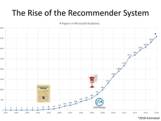
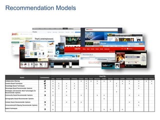
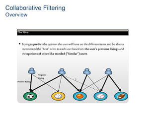
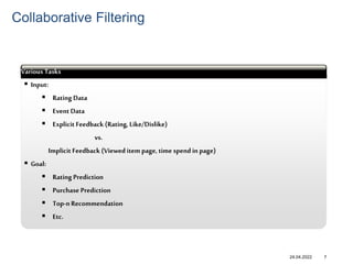
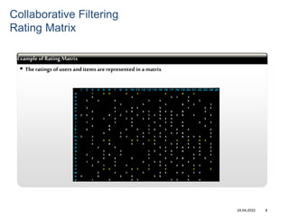
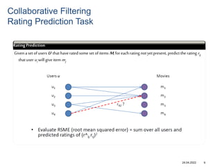
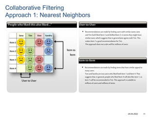
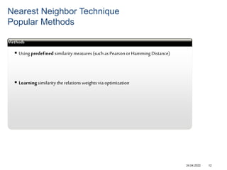
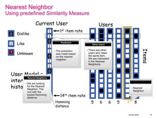
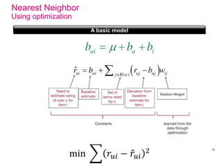
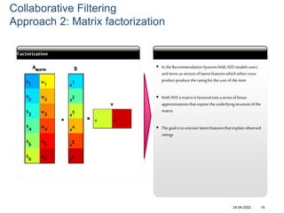
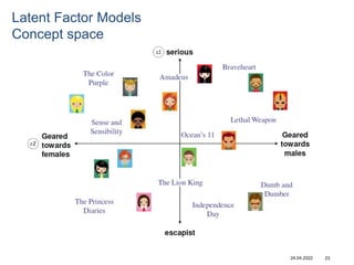
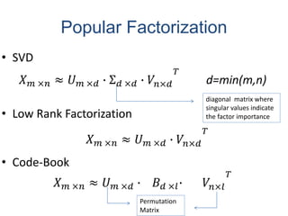
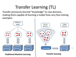
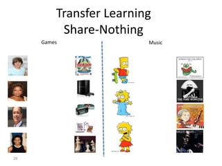
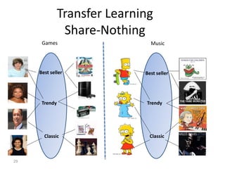
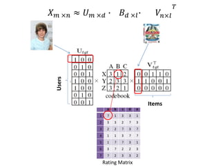
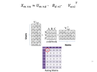
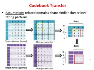
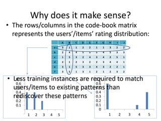
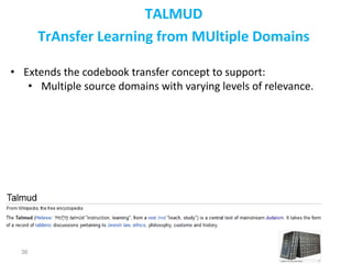
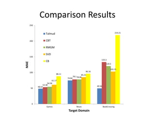
Recommender systems help users deal with overwhelming choices by providing personalized recommendations. They are commonly used by websites like Amazon, Netflix, and YouTube. Research on recommender systems has grown significantly over the past 20 years. Common recommendation models include collaborative filtering, which predicts ratings based on similar users or items, and matrix factorization, which represents users and items as vectors in a latent space. Transfer learning techniques allow knowledge from related domains to improve recommendations for new users or items.


![[DSC Europe 25] Andrzej Kowalczyk - AI - how to start small and grow in the f...](https://cdn.slidesharecdn.com/ss_thumbnails/oy1zmo94qv6vpcqjvno2-andrzej-kowalczyk-ai-how-to-start-small-and-grow-in-the-future-1-260119121559-cf093b23-thumbnail.jpg?width=640&height=640&fit=bounds)


![[DSC Europe 25] Elena Menshikova - AI-Powered Operational Excellence: Revolut...](https://cdn.slidesharecdn.com/ss_thumbnails/es6nholbqy3zaao2c2yd-2-elena-menshikova-data-ai-in-decision-making-260115093812-4fba8b38-thumbnail.jpg?width=640&height=640&fit=bounds)

