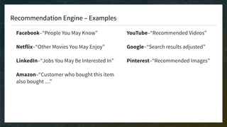
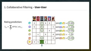
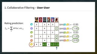
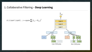
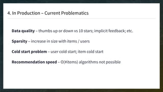
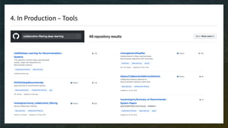
The document discusses recommendation engines, emphasizing the importance of addressing choice overload through collaborative filtering, content-based, and hybrid models. It highlights the challenges faced by collaborative filtering methods, such as sparsity and scalability, while proposing solutions to improve recommendation quality and performance. Additionally, it touches on current problems in production, including data quality, cold starts, and recommendation speed, along with potential tools to enhance these systems.

1. Thank you

2. 19 min searching
300 million viewers
5 billion hours wasted per year
at least once a week

3. 19 min searching
300 million viewers
5 billion hours wasted per year
at least once a week

5. Recommendation Engine
Information filtering systems
Deal with choice overload
Focused on user’s:
Preferences
Interest
Observed Behavior

6. Recommendation Engine – Examples
Facebook–“People You May Know”
Netflix–“Other Movies You May Enjoy”
LinkedIn–“Jobs You May Be Interested In”
Amazon–“Customer who bought this item
also bought …”
YouTube–“Recommended Videos”
Google–“Search results adjusted”
Pinterest–“Recommended Images”

7. Plan for Today
1. Collaborative Filtering
- User-User
- Item-Item
- User-Item
2. Content-Based
3. Hybrid Model
4. In Production

8. Collaborative Filtering

9. 1. Collaborative Filtering
recommend
buy
buy

10. 1. Collaborative Filtering – Rating Matrix
D( , ) = 4 ∈ {∅,1,2,3,4,5}
r. , = 4 − 3 = 1 ∈ {∅, -2,-1,0,1,2}
Rating data:
Re-centered rating data:

11. 1. Collaborative Filtering – Similarity Function
Real function that quantify the similarity between two objects.
1 − ||a − b||2 = 1 −
n
∑
i=1
(ai − bi)2
1 − ||a − b||1 = 1 −
n
∑
i=1
|ai − bi |
1 − ||a − b||p = 1 −
(
n
∑
i=1
|ai − bi |p
)
1/p
a⊤
b
||a||2 ||b||2
=
∑
n
i=1
aibi
∑
n
i=1
a2
i ∑
n
i=1
b2
i
sim(a, b) = …

12. 1. Collaborative Filtering – Similarity Function
Real function that quantify the similarity between two objects.
1 − ||a − b||2 = 1 −
n
∑
i=1
(ai − bi)2
1 − ||a − b||1 = 1 −
n
∑
i=1
|ai − bi |
1 − ||a − b||p = 1 −
(
n
∑
i=1
|ai − bi |p
)
1/p
a⊤
b
||a||2 ||b||2
=
∑
n
i=1
aibi
∑
n
i=1
a2
i ∑
n
i=1
b2
i
sim(a, b) = …

13. 1. Collaborative Filtering – User-User

14. 1. Collaborative Filtering – User-User
sim( , ) = -0.95

15. sim( , ) =
sim( , ) =
sim( , ) =
sim( , ) =
sim( , ) =
1. Collaborative Filtering – User-User
-0.95
1.00
0.00
-1.00
0.00

16. 1. Collaborative Filtering – User-User
sim( , ) =
sim( , ) =
sim( , ) =
sim( , ) =
sim( , ) = -0.95
1.00
0.00
-1.00
0.00

17. 1. Collaborative Filtering – User-User
̂yu,i =
∑
u′
sim(u′, u)ru′,i
Rating prediction:
4.0
sim( , ) =
sim( , ) =
sim( , ) =
sim( , ) =
sim( , ) = -0.95
1.00
0.00
-1.00
0.00

18. 1. Collaborative Filtering – User-User
̂yu,i =
∑
u′
sim(u′, u)ru′,i
Rating prediction:
4.0 1.0 1.5
sim( , ) =
sim( , ) =
sim( , ) =
sim( , ) =
sim( , ) = -0.95
1.00
0.00
-1.00
0.00

19. 1. Collaborative Filtering – User-User
̂yu,i =
∑
u′
sim(u′, u)ru′,i
Rating prediction:
Recommendation:
argmax
i
̂yu,i
1.0 1.54.0
sim( , ) =
sim( , ) =
sim( , ) =
sim( , ) =
sim( , ) = -0.95
1.00
0.00
-1.00
0.00

20. 1. Collaborative Filtering – User-User Benefits
- “People who bought that also bought that”
- Good when #items >> #users

21. 1. Collaborative Filtering – User-User Challenges
- Sparsity
- Don’t scale – Nearest Neighbors requires computation that grows with
the number of users and items
- Model Too Simplistic – Accuracy of recommendation may be poor

22. 1. Collaborative Filtering – Item-Item

23. 1. Collaborative Filtering – Item-Item
sim( , ) = -0.95
-0.95

24. 1. Collaborative Filtering – Item-Item
-1.00 -1.00 -0.95 1.00 0.00 1.00

25. 1. Collaborative Filtering – Item-Item
-0.95 -1.00 1.001.00-1.00 1
-1.00 -1.00 -0.95 1.00 0.00 1.00

26. 1. Collaborative Filtering – Item-Item
1.00 0.00 -1.00 0.00 -1.001
-0.95 -1.00 1.001.00-1.00 1
-1.00 -1.00 -0.95 1.00 0.00 1.00
⋮ ⋮ ⋮ ⋮ ⋮ ⋮ ⋮

27. 1. Collaborative Filtering – Item-Item
1.00 0.00 -1.00 0.00 -1.001
-0.95 -1.00 1.001.00-1.00 1
-1.00 -1.00 -0.95 1.00 0.00 1.00
⋮ ⋮ ⋮ ⋮ ⋮ ⋮ ⋮

28. 1. Collaborative Filtering – Item-Item
̂yu,i =
∑
i′
ru,i′ sim(i′, i)
1.00 0.00 -1.00 0.00 -1.001
-0.95 -1.00 1.001.00-1.00 1
-1.00 -1.00 -0.95 1.00 0.00 1.00
1.4 ⋮ ⋮ ⋮ ⋮ ⋮ ⋮ ⋮

29. 1. Collaborative Filtering – Item-Item
1.5 5.0
1.00 0.00 -1.00 0.00 -1.001
-0.95 -1.00 1.001.00-1.00 1
-1.00 -1.00 -0.95 1.00 0.00 1.00
1.4 ⋮ ⋮ ⋮ ⋮ ⋮ ⋮ ⋮
̂yu,i =
∑
i′
ru,i′ sim(i′, i)

30. 1. Collaborative Filtering – Item-Item
5.0
1.00 0.00 -1.00 0.00 -1.001
-0.95 -1.00 1.001.00-1.00 1
-1.00 -1.00 -0.95 1.00 0.00 1.00
5.01.4 1.5
̂yu,i =
∑
i′
ru,i′ sim(i′, i)
⋮ ⋮ ⋮ ⋮ ⋮ ⋮ ⋮

31. 1. Collaborative Filtering – Item-Item Benefits
- “If you like this you might also like that”
- Good when #users >> #items
- Very fast after the item-item table has been pre-computed

32. 1. Collaborative Filtering – Item-Item Challenges
- Bottleneck – similarity computation
- Space complexity – dense item-item similarity matrix
- Model Too Simplistic – Accuracy of recommendation may be poor

33. 1. Collaborative Filtering – User-Item

34. 1. Collaborative Filtering – User-Item

35. 1. Collaborative Filtering – User-Item
D(u,i) ≈ Uu
⊤
Ii =
∑
z
Uu,z Ii,z
D ≈ U⊤
I

36. 1. Collaborative Filtering – User-Item
…
… …
User Item
y!
u,i
D(u,i) ≈ Uu
⊤
Ii =
∑
z
Uu,z Ii,z
…
…
Uu Ii

37. 1. Collaborative Filtering – User-Item
…
… …
y!
u,i
(U, I) = argmin
∑ (U⊤
u Ii − D(u,i))
2
D(u,i) ≈ Uu
⊤
Ii =
∑
z
Uu,z Ii,z
User ItemUu Ii

38. 1. Collaborative Filtering – Matrix Factorization
ℒ(U, I) =
∑
u,i
(U⊤
u Ii − D(u,i))
2
≈ ||U⊤
I − D||2
F (U, I) = argmin ℒ(U, I)
- SGD – Stochastic Gradient Descent
Ub+1
← Ub
− η
∂ℒ(Ub
, Ib
)
∂Ub
Ib+1
← Ib
− η
∂ℒ(Ub
, Ib
)
∂Ib

39. 1. Collaborative Filtering – Matrix Factorization
ℒ(U, I) =
∑
u,i
(U⊤
u Ii − D(u,i))
2
≈ ||U⊤
I − D||2
F (U, I) = argmin ℒ(U, I)
- SGD – Stochastic Gradient Descent
- SVD – Truncated Singular Value Decomposition
Ub+1
← Ub
− η
∂ℒ(Ub
, Ib
)
∂Ub
Ib+1
← Ib
− η
∂ℒ(Ub
, Ib
)
∂Ib
D = VΣW ≈ V:kΣ:kW:k U⊤
← V:kΣ1/2
:k I ← W:kΣ1/2
:k

40. 1. Collaborative Filtering – Matrix Factorization
ℒ(U, I) =
∑
u,i
(U⊤
u Ii − D(u,i))
2
≈ ||U⊤
I − D||2
F (U, I) = argmin ℒ(U, I)
- SGD – Stochastic Gradient Descent
- SVD – Truncated Singular Value Decomposition
- ALS – Alternating Least Square
Ub+1
← Ub
− η
∂ℒ(Ub
, Ib
)
∂Ub
Ib+1
← Ib
− η
∂ℒ(Ub
, Ib
)
∂Ib
D = VΣW ≈ V:kΣ:kW:k U⊤
← V:kΣ1/2
:k I ← W:kΣ1/2
:k
Ub+1
← DIb
(Ib⊤
Ib
)−1
Ib+1
← DUb
(Ub⊤
Ub
)−1

41. 1. Collaborative Filtering – User-Item Benefits
similar
- Fast after U and I are pre-computed
- Can learn more about users with U
- Can learn more about items with I

42. 1. Collaborative Filtering – User-Item Challenges
- Sparsity
- Need to re-learn everything every time a new user or new item or new
rating enter the game
- Only linear prediction

43. 1. Collaborative Filtering – Sparsity Example, the Netflix Prize
- 17,770 Movies
- 480,189 Users
- 100,480,507 Ratings
How dense is our Matrix ?
Ratings
Movies ×Users
=
100,480,507
17,770 × 480,189
×100 = 1.18%

44. 1. Collaborative Filtering – Sparsity Example, the Netflix Prize
- 17,770 Movies
- 480,189 Users
- 100,480,507 Ratings
How dense is our Matrix ?
Ratings
Movies ×Users
=
100,480,507
17,770 × 480,189
×100 = 1.18%
users
movies

45. 1. Collaborative Filtering – Deep Learning
- Non-linear interactions
- Enable transfer learning on multiple dataset
- Enable to use meta-data (keywords, tags)
- Enable to use graph-based data (those who like movies with this actor also
like movies with this other actor)

46. 1. Collaborative Filtering – Deep Learning
…
… …
Layer 3
Layer 2
Layer 1
pooling pooling
u g1 g2
1 3.2 … 0 0
User Attributes
g2 g4 g5i
0 1 … 1 2.0
Item Attributes
̂yu,i
̂yu,i

47. 1. Collaborative Filtering – Deep Learning
(U, I, Layer1, Layer2, …) = argmin
∑ ( ̂yu,i − D(u,i))
2
Layer 3
Layer 2
Layer 1
pooling pooling
u g1 g2 g2 g4 g5i
̂yu,i
1 3.2 … 0 0
User Attributes
0 1 … 1 2.0
Item Attributes

48. 1. Collaborative Filtering – Deep Learning
(U, I, Layer1, Layer2, …) = argmin
∑ ( ̂yu,i − D(u,i))
2
- “Mini”-Batch Stochastic Gradient Descent
- Acceleration Heuristics (AdaGrad, Nesterov, RMSprop, Adam, NAdam, ...)
- DropOut / BatchNorm
- Watch-out for Sparse Data and Momentum! vs
- Hyper-parameters Optimization
ru,i = 0 ru,i = ∅

49. Content Extraction

50. 2. Content Extraction
Based on “what does the user like
about an item”:
- Meta-data extraction
- Clustering
- Similarity/distance between objects
likely buy
buy

51. 2. Content Extraction – Item-Item Similarity
- Allow to compute similarities between items
- Does not require rating dataset
- The previous item-item recommendation algorithm still works
- No item cold start
- User attributes mitigate user cold start

52. 2. Content Extraction – Deep
Every single item is not just about
the available meta-data.
Encode information from:
- Images (CNN)
- Text Information (NLP)
- Audio (LSTM)
Input
A documentary which
examines the creation and
co-production of the
popular children’s
television program in three
developing countries:
Bangladesh, Kosovo, and
South Africa.
Prediction
Comedy,
Adventure,
Family,
Animation
In his spectacular film
debut, young Babar, King
of the Elephants must
save his homeland from
certain destruction by
Rataxes and his band of
invading rhinos.
Documentary,
History
Comedy,
Adventure,
Family,
Animation
Adventure, War,
Documentary,
Music

53. Hybrid Model

54. 3. Hybrid Model
Layer 3
Layer 2
Layer 1
pooling
u g1 g2
1 1 … 0 0
User Attributes
g2 g4 g5i
0 1 … 1 1
Item Attributes
g100 g… g… g… g200 g… g…
A documentary which examines
the creation and co-production of
the popular children’s television
program in three developing
countries: Bangladesh, Kosovo,
and South Africa.
g…
pooling
g… g…
̂yu,i

55. 3. Hybrid Model
Layer 3
Layer 2
Layer 1
pooling
u g1 g2
1 1 … 0 0
User Attributes
g2 g4 g5i
0 1 … 1 1
Item Attributes
g100 g… g… g… g200 g… g…
A documentary which examines
the creation and co-production of
the popular children’s television
program in three developing
countries: Bangladesh, Kosovo,
and South Africa.
g…
pooling
g… g…
̂yu,i
pre-computed as input
fully trained in SGD

56. 3. Hybrid Model
- The previous deep learning recommendation algorithm still works
- Improve recommendations of items without many ratings
- Mitigate item cold start
- Mitigate user cold start
- Improve transfer learning

57. In Production

58. 4. In Production – Current Problematics
Data quality – thumbs up or down vs 10 stars; implicit feedback; etc.
Sparsity – increase in size with items / users
Cold start problem – user cold start; item cold start
Recommendation speed – O(#items) algorithms not possible

59. 4. In Production – Solutions
Data quality
Unbiased consumer app where the users enter their tastes
Sparsity
User interaction: Ask each user to rate the most informative items
Cold start problem
Hybrid models with deep content extraction to recommend new items without ratings
Recommendation speed
Use item-item rec-sys with pre-computed item similarities to compute a (large) set of
candidates; compute feedforward neural network on candidates only

60. 4. In Production – Tools
LightFM
🙂 open source: https://github.com/lyst/lightfm
🙂 hybrid: matrix factorization + context
😐 linear
Deep Learning?
😐 way less tools than Computer Vision or NLP
😐 no pre-trained model available – you need large dataset and GPUs
😐 TensorFlow and PyTorch support for sparse data is limited

61. 4. In Production – Tools

62. 4. In Production – Tools

63. 4. In Production – Cloud Based
Do you want to hear more?
Let's get in touch with us at Crossing Minds!
We are building an API to offer state-of-the-art recommendations on the cloud

64. Thank you