Downloaded 383 times


![Quick sort
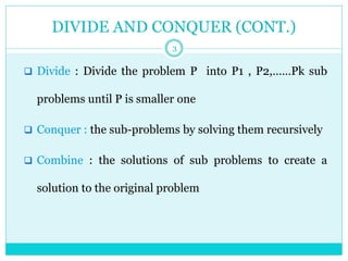
1. Divide: partition A[p..r] into two sub arrays A[p..q-1] and
A[q+1..r] such that each element of A[p..q-1] is ≤ A[q],
and each element of A[q+1..r] is ≥ A[q]. Compute q as part
of this partitioning.
2. Conquer: sort the sub arrays A[p..q-1] and A[q+1..r] by
recursive calls to QUICKSORT.
3. Combine: the partitioning and recursive sorting leave us
with a sorted A[p..r]
9](https://image.slidesharecdn.com/divideandconquer-161111094807/85/Divide-and-conquer-Quick-sort-9-320.jpg)
![Quick sort algorithm
QUICKSORT(A[p,…r])
Input: A[p,….r]
Output: the sub array A[1…r] stored in non decreasing order
If p<r
q= PARTITION(A,p,r)
QUICKSORT(A[p,q-1])
QUICKSORT(A[q+1, r])
10
v
v
S1 S2
S](https://image.slidesharecdn.com/divideandconquer-161111094807/85/Divide-and-conquer-Quick-sort-10-320.jpg)
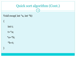
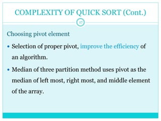
![Quick sort algorithm (Cont.)
11
PARTITION(A[p…r])
Initialization
P=A[p]
i=p
j=r+1](https://image.slidesharecdn.com/divideandconquer-161111094807/85/Divide-and-conquer-Quick-sort-11-320.jpg)
![Quick sort algorithm (Cont.)
12
Repeat
Repeat i=i+1 until A[i]≥P
Repeat j=j-1 until A[j]≤P
Swap(A[i],A[j])
Until i ≥ j
Swap(A[p],a[j]);
Return j](https://image.slidesharecdn.com/divideandconquer-161111094807/85/Divide-and-conquer-Quick-sort-12-320.jpg)
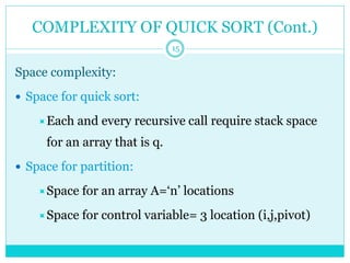
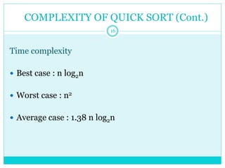
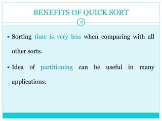


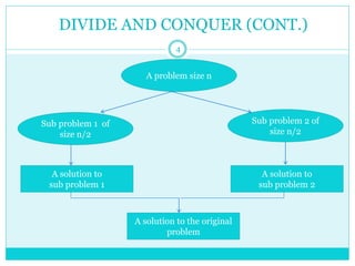
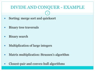
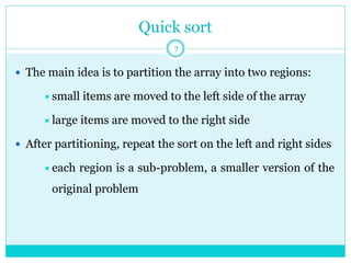
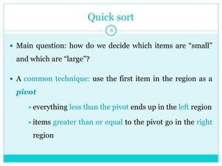
The document explains the divide and conquer strategy in algorithms, emphasizing its recursive nature and applications in sorting methods like quicksort and merge sort. Quicksort operates by partitioning arrays into smaller regions based on a pivot element to efficiently sort them. It outlines the algorithm's complexities, benefits, and techniques for choosing an effective pivot to enhance performance.


![ppt daaa[1].pptxdaaaaaaaaaaaaaaaaaaaaaaaaaaaaaaaaa](https://cdn.slidesharecdn.com/ss_thumbnails/pptdaaa1-251211161628-1cb28a51-thumbnail.jpg?width=640&height=640&fit=bounds)


![UNIT V Searching Sorting Hashing Techniques [Autosaved].pptx](https://cdn.slidesharecdn.com/ss_thumbnails/unitvsearchingsortinghashingtechniquesautosaved-241126054304-95a69c51-thumbnail.jpg?width=640&height=640&fit=bounds)
![UNIT V Searching Sorting Hashing Techniques [Autosaved].pptx](https://cdn.slidesharecdn.com/ss_thumbnails/unitvsearchingsortinghashingtechniquesautosaved-241014040608-74caa0f6-thumbnail.jpg?width=640&height=640&fit=bounds)