This document provides examples of simulating queueing systems using discrete-event simulation. It summarizes a single-channel queue simulation where customers arrive randomly and have randomly distributed service times. Next, it simulates a grocery store with one checkout counter to analyze customer wait times. Finally, it simulates a call center with two agents (Abel and Baker) that handles 100 calls, tracking customer arrival times, service agents, and time in system to analyze system performance. Key outputs include total time in system, average wait times, and agent idle times.

1. Chapter 2
Simulation Examples
Banks, Carson, Nelson & Nicol
Discrete-Event System Simulation

2. Purpose
 To present several examples of simulations that can be
performed by devising a simulation table either manually
or with a spreadsheet.
 The simulation table provides a systematic method for
tracking the system state over time.
 To provide insight into the methodology of discrete-
system simulation and the descriptive statistics used for
predicting system performance.
2

3. Outline
 The simulations are carried out by following steps:
 Determine the input characteristics.
 Construct a simulation table.
 For each repetition i, generate a value for each input, evaluate
the function, and calculate the value of the response yi.
 Simulation examples are in queueing, inventory, reliability
and network analysis. 3

4. Simulation of Queueing Systems
 A queueing system is described by its calling population, nature of
arrivals, service mechanism, system capacity and the queueing
discipline (details in Chapter 6.)
 In a single-channel queue:
 The calling population is infinite.
 Arrivals for service occur one at a time in a random fashion, once they
join the waiting line, they are eventually served.
 Arrivals and services are defined by the distribution of the time
between arrivals and service times.
 Key concepts:
 System state is the number of units in the system and the status of the
server (busy or idle).
 An event is a set of circumstances that causes an instantaneous
change in the system state, e.g., arrival and departure events.
 The simulation clock is used to track simulated time.
4

5. Simulation of Queueing Systems
 Event list: to help determine what happens next.
 Tracks the future times at which different types of events occur.
(this chapter simplifies the simulation by tracking each unit
explicitly)
 Events usually occur at random times.
 The randomness needed to imitate real life is made possible
through the use of random numbers, they can be generated
using:
 Random digits tables: form random numbers by selecting the
proper number of digits and placing a decimal point to the left of
the value selected, e.g., Table A.1 in book.
 Simulation packages and spreadsheets.
 Details in chapter 7.
5

6. Simulation of Queueing Systems
6
System State: # of entities in the system & Server Status
(busy/idle)
Events: arrival & departure
Simulation Clock: variable representing simulated time.
Simulation clock is used to track simulation time.

7. Arrival Event
7

8. Departure Event
8

9. Simulation of Queueing Systems
9

10. Simulation of Queueing Systems
 Single-channel queue illustration:
 Assume that the times between arrivals were generated by rolling
a die 5 times and recording the up face. Input generated:
 The 1st
customer is assumed to arrive at clock time 0. 2nd
customer
arrives two time units later (at clock time 2), and so on.
 Assume the only possible service times are 1, 2, 3 and 4 time
units and they are equally likely to occur. Input generated:
Customer Interarrival Time Arrival Time on Clock
1 - 0
2 2 2
3 4 6
4 1 7
5 2 9
6 6 15
Customer Service Time Customer Service Time
1 2 4 2
2 1 5 1
3 3 6 4
10

11. Simulation of Queueing Systems
 Resulting simulation table emphasizing clock times:
 Another presentation method, by chronological ordering of events:
Customer
Number
Arrival Time
(clock)
Time Service
Begins (Clock)
Service Time
(Duration)
Time Service
Ends (clock)
1 0 0 2 2
2 2 2 1 3
3 6 6 3 9
4 7 9 2 11
5 9 11 1 12
6 15 15 4 19
Event Type Customer Number Clock Time
Arrival 1 0
Departure 1 2
Arrival 2 2
Departure 2 3
Arrival 3 6
Arrival 4 7
Departure 3 9
Arrival 5 9
Departure 4 11
Departure 5 12
Arrival 6 15
Departure 6 19
11

12. Simulation of Queueing Systems
 Grocery store example: with only one checkout counter.
 Customers arrive at random times from 1 to 8 minutes apart, with
equal probability of occurrence:
 The service times vary from 1 to 6 minutes, with probabilities:
Time between
Arrivals (minutes) Probability
Cumulative
Probability
Random Digit
Assignment
1 0.125 0.125 001-125
2 0.125 0.250 126-250
3 0.125 0.375 251-375
4 0.125 0.500 376-500
5 0.125 0.625 501-625
6 0.125 0.750 626-750
7 0.125 0.875 751-875
8 0.125 1.000 876-000
Time between
Arrivals (minutes) Probability
Cumulative
Probability
Random Digit
Assignment
1 0.10 0.100 001-100
2 0.20 0.300 101-300
3 0.30 0.600 301-600
4 0.25 0.850 601-850
5 0.10 0.950 851-950
6 0.05 1.000 951-000
12

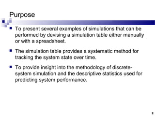
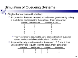
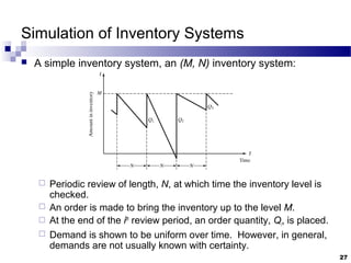
13. Grocery Store Example
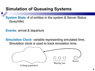
[Simulation of Queueing Systems]
 To analyze the system by simulating arrival and service of 100
customers.
 Chosen for illustration purpose, in actuality, 100 customers is too small a
sample size to draw any reliable conclusions.
 Initial conditions are overlooked to keep calculations simple.
 A set of uniformly distributed random numbers is needed to generate
the arrivals at the checkout counter:
 Should be uniformly distributed between 0 and 1.
 Successive random numbers are independent.
 With tabular simulations, random digits can be converted to random
numbers.
 List 99 random numbers to generate the times between arrivals.
 Good practice to start at a random position in the random digit table and
proceed in a systematic direction (never re-use the same stream of digits
in a given problem.
13

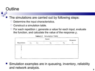
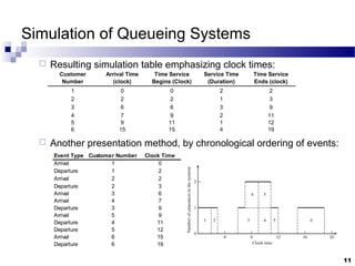
14. Grocery Store Example
[Simulation of Queueing Systems]
 Generated time-between-arrivals:
 Using the same methodology, service times are generated:
Customer Random Digits Interarrival Times (minutes)
1 - -
2 64 1
3 112 1
4 678 6
5 289 3
6 871 7
… … …
100 538 4
Customer Random Digits Service Times (minutes)
1 842 4
2 181 2
3 873 5
4 815 4
5 006 1
6 916 5
100 266 2
14

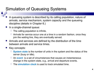
15. Grocery Store Example
[Simulation of Queueing Systems]
 For manual simulation, Simulation tables are designed for the
problem at hand, with columns added to answer questions
posed:
Customer
Interarrival
Time (min)
Arrival
Time
(clock)
Service
Time
(min)
Time
Service
Begins
(clock)
Waiting
Time in
Queue
(min)
Time
Service
Ends
(clock)
Time
customer
spends in
system (min)
Idle time
of server
(min)
1 0 4 0 0 4 4
2 1 1 2 4 3 6 5 0
3 1 2 5 5 4 11 9 0
4 6 8 4 11 3 15 7 0
5 3 11 1 15 4 16 5 0
6 7 18 5 18 0 23 5 2
… … … … … … … … …
100 5 415 2 416 1 418 3
Totals 415 317 174 491 0
15
Service could not begin until
time 4 (server was busy until
that time)
2nd customer was in the system for
5 minutes.
Service ends at time 16, but
the 6th customer did not arrival
until time 18. Hence, server
was idle for 2 minutes

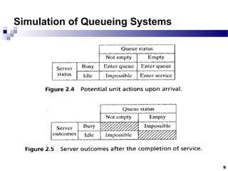
16. Grocery Store Example
[Simulation of Queueing Systems]
 Tentative inferences:
 About half of the customers have to wait, however, the average waiting
time is not excessive.
 The server does not have an undue amount of idle time.
 Longer simulation would increase the accuracy of findings.
 Note: The entire table can be generated using the Excel spreadsheet
for Example 2.1 at www.bcnn.net
16

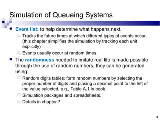
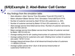
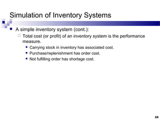
17. Grocery Store Example
[Simulation of Queueing Systems]
 Key findings from the simulation table:
min5.42/)81(timealinterarrivExpected:Check
min19.4
99
415
1arrivalsofnumber
(min)timesalinterarrivallofsum
(min)Times
alinterarrivAverage
min2.3
)05.0(6)1.0(5)25.0(4)3.0(3)2.0(2)1.0(1
timeserviceExpected:Check
min17.3
100
317
customersofnumbertotal
(min)timeservicetotal
(min)time
serviceAverage
0.760.24-1serverbusyofyProbabilit:Hence
24.0
418
101
(min)simulationofrun timetotal
(min)serveroftimeidletotal
serveridle
ofyProbabilit
46.0
100
46
customersofnumbertotal
waitwhocustomersofnumbers
y(wait)Probabilit
min74.1
100
174
customersofnumbertotal
(min)queueinwaittimetotal
(min)time
waitingAverage
=+=
==
−
=
=
+++++=
===
==
===
===
===
17

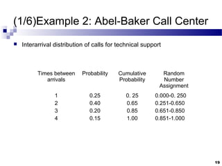
18. Able-Baker Call Center Example
[Simulation of Queueing Systems]
 A computer technical support center with two personnel
taking calls and provide service.
 Two support staff: Able and Baker (multiple support channel).
 A simplifying rule: Able gets the call if both staff are idle.
 Goal: to find how well the current arrangement works.
 Random variable:
 Arrival time between calls
 Service times (different distributions for Able and Baker).
 A simulation of the first 100 callers are made
 More callers would yield more reliable results, 100 is chosen for
purposes of illustration.
18

19. (1/6)Example 2: Abel-Baker Call Center
 Interarrival distribution of calls for technical support
Times between
arrivals
Probability Cumulative
Probability
Random
Number
Assignment
1
2
3
4
0.25
0.40
0.20
0.15
0. 25
0.65
0.85
1.00
0.000-0. 250
0.251-0.650
0.651-0.850
0.851-1.000
19

20. (2/6)Example 2: Abel-Baker Call Center
 Service times Distribution of Abel
Service Times Probability Cumulative
Probability
Random Number
Assignment
2
3
4
5
0.30
0.28
0.25
0.17
0.3
0.58
0.83
1.00
0.000-0.300
0.301-0.580
0.581-0.830
0.831-1.000
20

21. (3/6)Example 2: Abel-Baker Call Center
 Service Time Distribution of Baker
Service Times Probability Cumulative
Probability
Random Number
Assignment
3
4
5
6
0.35
0.25
0.20
0.20
0.35
0.60
0.80
1.00
0.000-0.350
0.351-0.600
0.601-0.800
0.801-1.000
21

22. (4/6)Example 2: Abel-Baker Call Center
 Simulation Table
Abel Baker
Customer
Number
arrival
Random
Number
Time
Between
Arrivals
Clock
time of
arrivals
Services
Random
Number
Service
time
start
Service
time
Service
time
ends
Servic
e time
start
S. T. S. T.
Ends
Time in
Queue
1
2
3
4
5
6
7
8
9
10
11
12
13
14
15
0.99284
0.46349
0.65493
0.00801
0.01753
0.02711
0.29430
0.70327
0.30517
0.02915
0.29487
0.84654
0.99127
0.68425
0.64327
4
2
3
1
1
1
2
3
2
1
2
3
4
3
2
4
6
9
10
11
12
14
17
19
20
22
25
29
32
34
0.39824
0.48585
0.01847
0.37545
0.38022
0.07169
0.79473
0.04861
0.74483
0.08278
0.91326
0.62540
0.98713
0.64157
0.41684
4
-
9
-
11
14
-
17
19
-
23
-
29
-
34
3
-
2
-
3
2
-
2
4
-
5
-
5
-
3
7
-
11
-
14
16
-
19
23
-
28
-
34
-
37
-
6
-
10
-
-
14
-
-
20
-
25
-
32
-
-
4
-
4
-
-
5
-
-
3
-
5
-
5
-
-
10
-
14
-
-
19
-
-
23
-
30
-
37
-
0
0
0
0
0
2
0
0
0
0
1
0
0
0
0
22

23. (5/6)Example 2: Abel-Baker Call Center
Abel Baker
Customer
Number
arrival
Random
Number
Time
Between
Arrivals
Clock
time of
arrivals
Services
Random
Number
Service
time
start
Service
time
Service
time
ends
Service
time
start
S.
T.
S. T.
Ends
Time in
Queue
16
17
18
19
20
21
22
23
24
25
26
27
28
29
30
0.36920
022224
0.43799
0.11914
0.66299
0.28891
0.90375
0.94859
0.37528
0.27395
0.66487
0.12508
0.80400
0.43157
0.78568
2
1
2
1
3
2
4
4
2
2
3
1
3
2
3
36
37
39
40
43
45
49
53
55
57
60
61
64
66
69
0.91637
0.71243
0.77096
0.06115
0.93464
0.92325
0.35555
0.68290
0.37974
0.27307
0.35881
0.83147
0.73653
0.75574
0.38987
37
-
42
-
-
46
51
-
55
58
60
-
64
-
69
5
-
4
-
-
5
3
-
3
2
3
-
4
-
3
42
-
46
-
-
51
54
-
58
60
63
-
68
-
72
-
37
-
42
45
-
-
53
-
-
-
61
-
67
-
-
5
-
3
6
-
-
5
-
-
-
6
-
5
-
-
42
-
45
51
-
-
58
-
-
-
67
-
72
-
1
0
3
2
2
1
2
0
0
1
0
0
0
1
0
Total 69 61 56 16
23

24. (6/6)Example 2: Abel-Baker Call Center
 Key findings from the simulation table:
 Abel utilization= (Abel Service Time /Simulation Time)=(61/72)=0.847 %
 Baker utilization=(Baker Service Time / Simulation Time)=(56/72)=0.777%
 Number of customer serviced by Abel=18 from (30 customers) i.e., 60%
 Number of customer serviced by Baker=12 from (30 customers) i.e., 40%
 Abel average service time=(Abel service time) / Number of customer serviced by
Abel =61/18=3.39 min
 Baker average service time=(Baker service time)/ Number of customer serviced
by Baker =56/12=4.46 min
 Average waiting time for all= (waiting time/number of customer)=(16/30)=0.53min
 Average waiting time for customers who wait= (Waiting time/ number of customer
who wait)= 16/10=1.6 min
 Average interarrival times=(Sum of all interarrival times)/number of customers
-1= 69/29=2.379 min
 Average system service time= (Sum of all service times/number of
customers)=72/30=2.4 min
24

25. Able-Baker Call Center Example
[Simulation of Queueing Systems]
 The steps of simulation are implemented in a spreadsheet
available on the website (www.bcnn.net).
 In the first spreadsheet, we found the result from the trial:
 62% of the callers had no delay
 12% had a delay of one or two minutes.
25

26. Able-Baker Call Center Example
[Simulation of Queueing Systems]
 In the second spreadsheet, we run an experiment with 400 trials
(each consisting of the simulation of 100 callers) and found the
following:
 19% of the average delays are longer than two minutes.
 Only 2.75% are longer than 3 minutes.
26

27. Simulation of Inventory Systems
 A simple inventory system, an (M, N) inventory system:
 Periodic review of length, N, at which time the inventory level is
checked.
 An order is made to bring the inventory up to the level M.
 At the end of the ith
review period, an order quantity, Qi, is placed.
 Demand is shown to be uniform over time. However, in general,
demands are not usually known with certainty.
27

28. Simulation of Inventory Systems
 A simple inventory system (cont.):
 Total cost (or profit) of an inventory system is the performance
measure.
 Carrying stock in inventory has associated cost.
 Purchase/replenishment has order cost.
 Not fulfilling order has shortage cost.
28

29. Simulation of Inventory Systems
 The News Dealer’s Example: A classical inventory
problem concerns the purchase and sale of newspapers.
 News stand buys papers for 33 cents each and sells them for 50
cents each.
 Newspaper not sold at the end of the day are sold as scrap for 5
cents each.
 Newspaper can be purchased in bundles of 10 (can only buy 10,
20,… 50, 60…)
 Random Variables:
 Types of newsdays.
 Demand.
Profits = (revenue from sales) – (cost of newspaper)
– (lost profit form excess demand)
+ (salvage from sale of scrap papers)
29

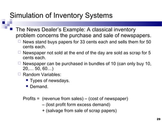
30. News Dealer’s Example
[Simulation of Inventory Systems]
 Three types of newsdays: “good”; “fair”; “poor”; with
probabilities of 0.35, 0.45 and 0.20, respectively.
 Distribution of newspaper demand
Type of Newsday Probability Cumulative Probability Random digit Assignment
Good 0.35 0.35 01-35
Fair 0.45 0.80 36-80
Poor 0.20 1.00 81-00
30

31. News Dealer’s Example
[Simulation of Inventory Systems]
 Demand and the random digit assignment is as follow:
Demand Good Fair Poor Good Fair Poor
40 0.03 0.10 0.44 01-03 01-10 01-44
50 0.08 0.28 0.66 04-08 11-28 45-66
60 0.23 0.68 0.82 09-23 29-68 67-82
70 0.43 0.88 0.94 24-43 69-88 83-94
80 0.78 0.96 1.00 44-78 89-96 95-00
90 0.93 1.00 1.00 79-93 97-00
100 1.00 1.00 1.00 94-00
Cumulative Distribution Random Digit Assignment
31

32. News Dealer’s Example
[Simulation of Inventory Systems]
 Simulate the demands for papers over 20-day time period to
determine the total profit under a certain policy, e.g. purchase
70 newspaper
 The policy is changed to other values and the simulation is
repeated until the best value is found.
32

33. News Dealer’s Example
[Simulation of Inventory Systems]
 From the manual solution
 The simulation table for the decision to purchase 70 newspapers
is for 20 days:
Day
Random
Digits for
Type of
Newsday
Type of
Newsday
Random
Digits for
Demand Demand
Revenue
from Sales
Lost Profit
from
Excess
demand
Salvage
from Sale
of Scrap Daily Profit
1 58 Fair 93 80 $35.00 $1.70 - $10.20
2 17 Good 63 80 $35.00 $1.70 - $10.20
3 21 Good 31 70 $35.00 - - $11.90
4 45 Fair 19 50 $25.00 - $1.00 $2.90
5 43 Fair 91 80 $35.00 $1.70 $10.20
… … … … … … … … …
19 18 Good 44 80 $35.00 $1.70 - $10.20
20 98 Poor 13 40 $20.00 - $1.50 -$1.60
$600.00 $17.00 $10.00 $131.90Total
33

34. News Dealer’s Example
[Simulation of Inventory Systems]
 From Excel: running the simulation for 400 trials (each for 20
days)
 Average total profit = $137.61.
 Only 45 of the 400 results in a total profit of more than $160.
34

35. News Dealer’s Example
[Simulation of Inventory Systems]
 The manual solution had a profit of $131.00, not far from the
average over 400 days, $137.61.
 But the result for a one-day simulation could have been the
minimum value or the maximum value.
 Hence, it is useful to conduct many trials.
 On the “One Trial” sheet in Excel spreadsheet of Example 2.3.
 Observe the results by clicking the button ‘Generate New Trail.’
 Notice that the results vary quite a bit in the profit frequency graph
and in the total profit.
35

36. Order-Up-To Level Inventory Example
[Simulation of Inventory Systems]
 A company sells refrigerators with an inventory system
that:
 Review the inventory situation after a fixed number of days (say
N) and order up to a level (say M).
Order quantity = (Order-up-to level) - (Ending inventory)
+ (Shortage quantity)
 Random variables:
 Number of refrigerators ordered each day.
 Lead time: the number of days after the order is placed with the
supplier before its arrival.
 See Excel solution for Example 2.4 for details.
36

37.  Set M (order up to level) =11 items
 Set the review period n= 5 days
Random digit assignments for lead
time
Random digit assignments for daily demand
37
Order-Up-To Level Inventory Example
[Simulation of Inventory
Systems]

38. 38
Order-Up-To Level Inventory Example
[Simulation of Inventory
Systems]
 Simulation table for (M=11, N=5) inventory System

39. 39
Order-Up-To Level Inventory Example
[Simulation of Inventory
Systems]
 Frequency distribution of average ending inventory for
100 trials (each 25 days)

40. Other Examples of Simulation
 Reliability problem:
 A machine with different failure types of which repairman is called
to install or repair the part.
 Possible random variables: time to failure, time to service.
 Possible decision variables: decide strategy of repair verses
replace, number of repairman to hire.
 Random normal numbers:
 e.g. a bomber problem – where the point of impact is normally
distributed around the aim point.
 Possible decision variables: number of bombs to drop for a certain
level of damage.
40

41. Other Examples of Simulation
 Lead-time demand:
 Lead time is the random variable: the time from placement of an
order until the order is received.
 Other possible random variable: demand.
 Possible decision variables: how much and how often to order.
 Project simulation:
 A project can be represented as a network of activities: some
activities must be carried out sequentially, others can be done in
parallel.
 Possible random variables: times to complete the activities.
 Possible decision variables: sequencing of activities, number of
workers to hire.
41

42. Summary
 Introduced simulation concepts by means of examples,
illustrated general areas of application, and motivated the
remaining chapters.
 Ad-hoc simulation tables were used:
 Events in tables were generated by using uniformly distributed
random numbers, and resulting responses were analyzed.
 Ac-hoc simulation table may fail due to system complexities.
More systematic methodology, e.g., event scheduling approach,
is described in Chapter 3.
 Key takeaways:
 A simulation is a statistical experiment and results have variation.
 As the number of replications increases, there is an increased
opportunity for greater variation.
42