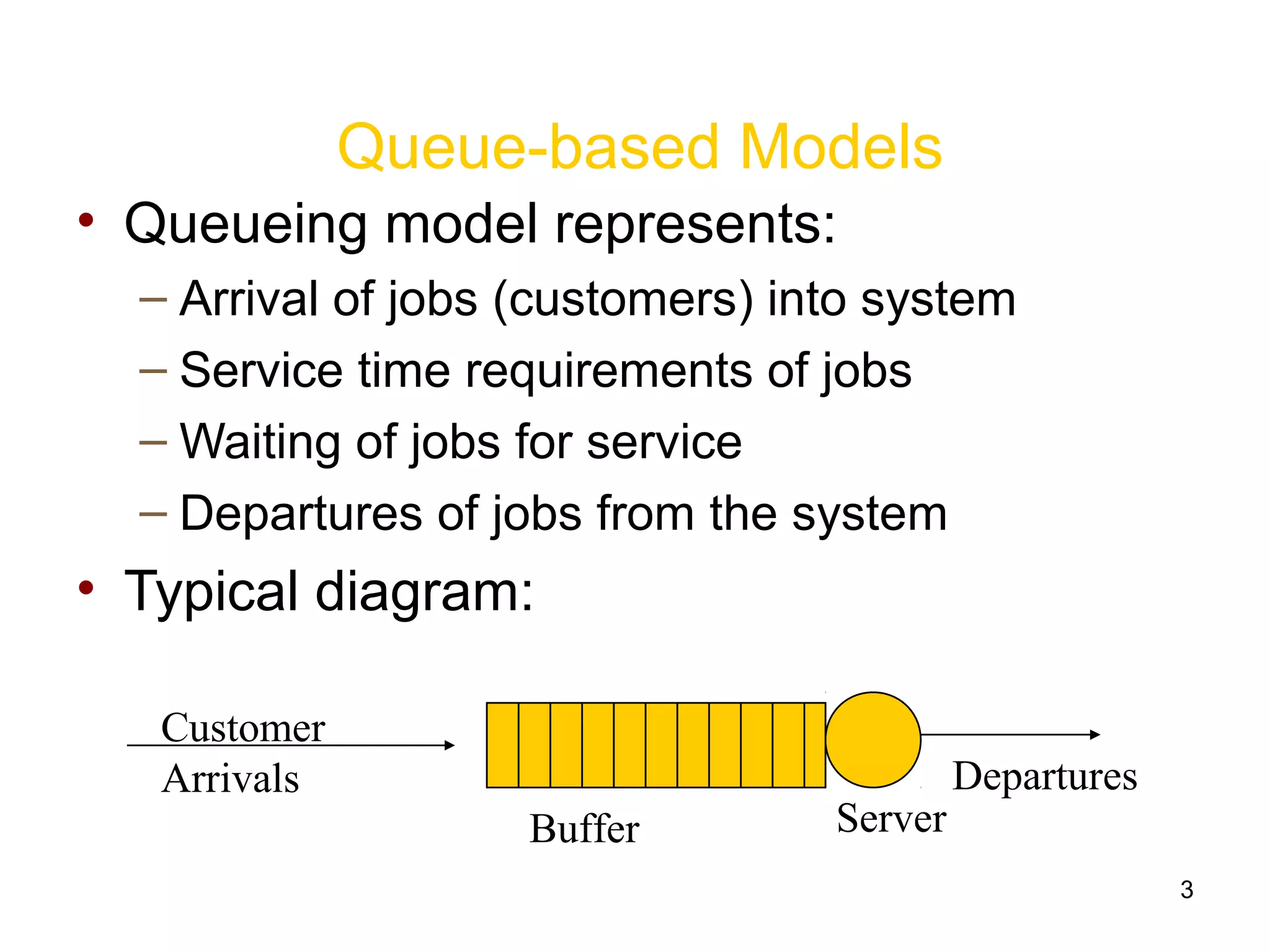
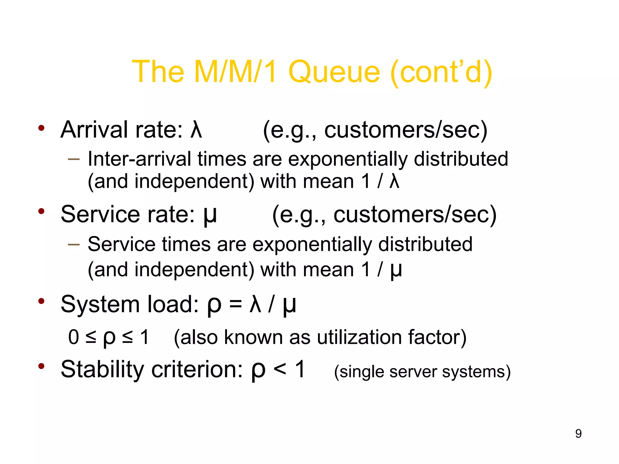
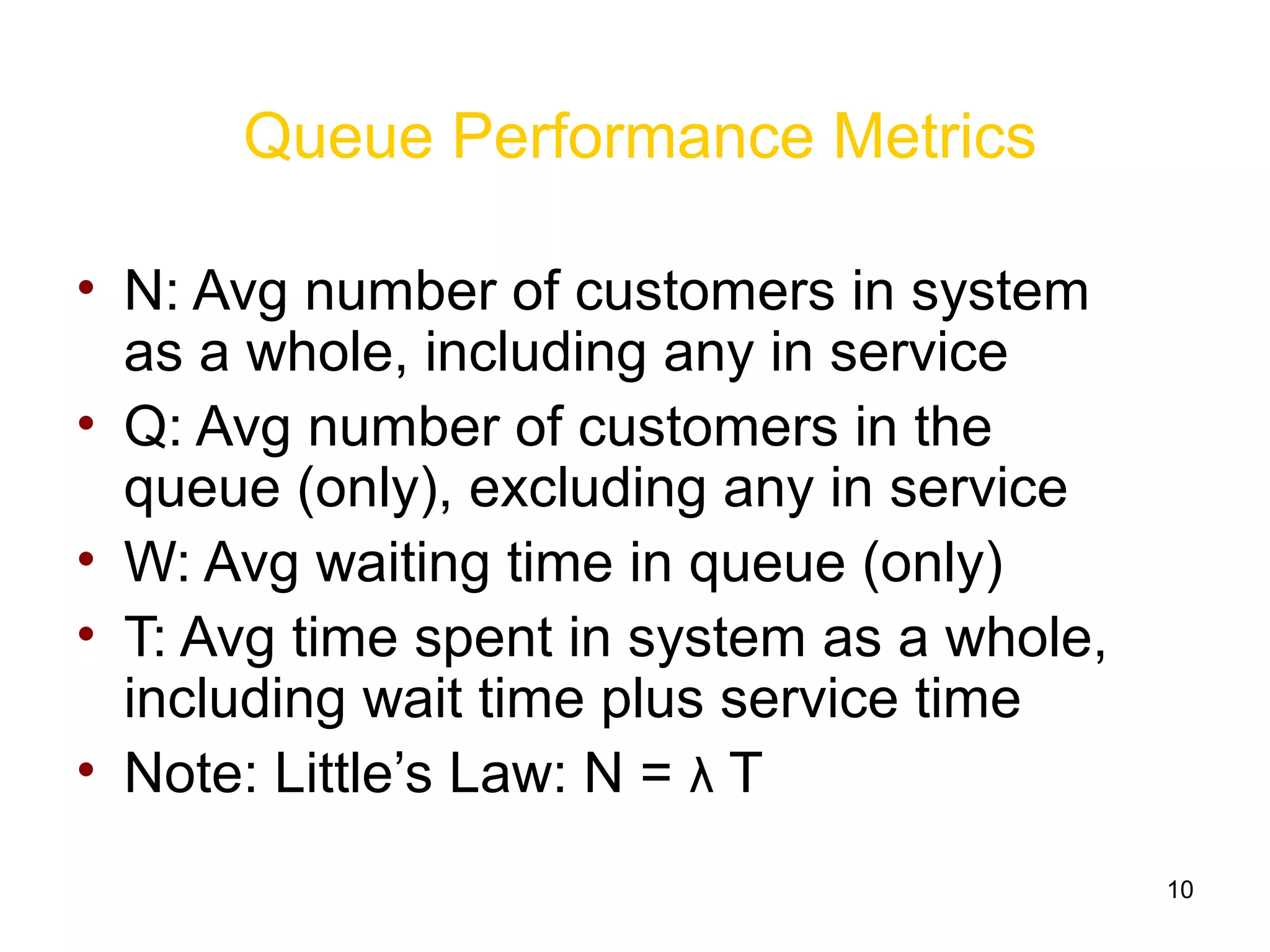
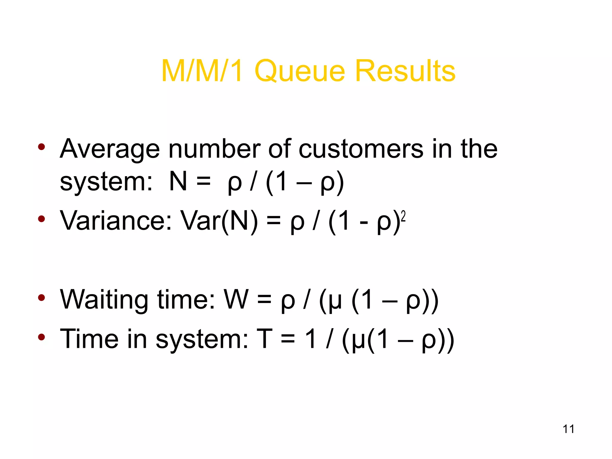
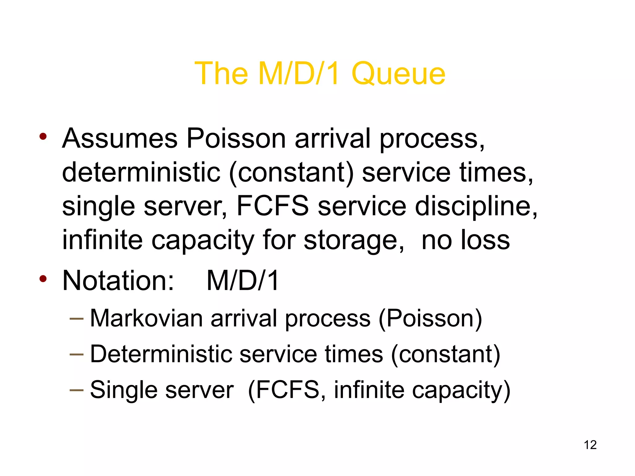
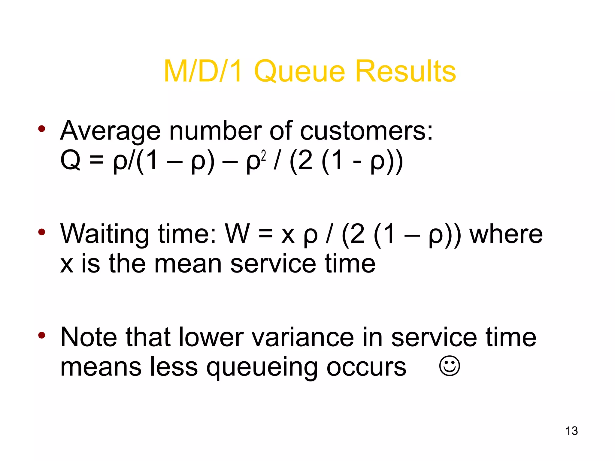
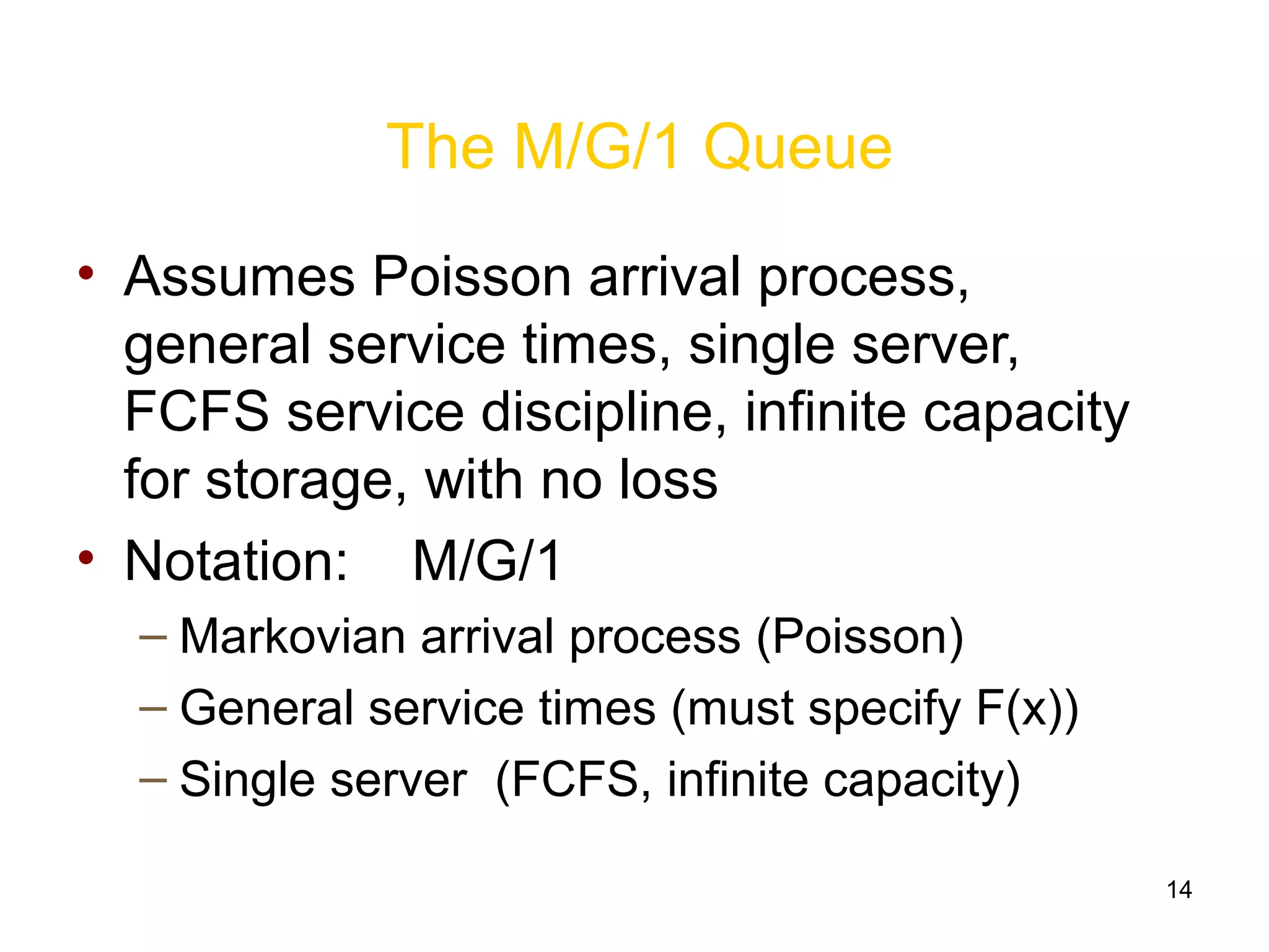
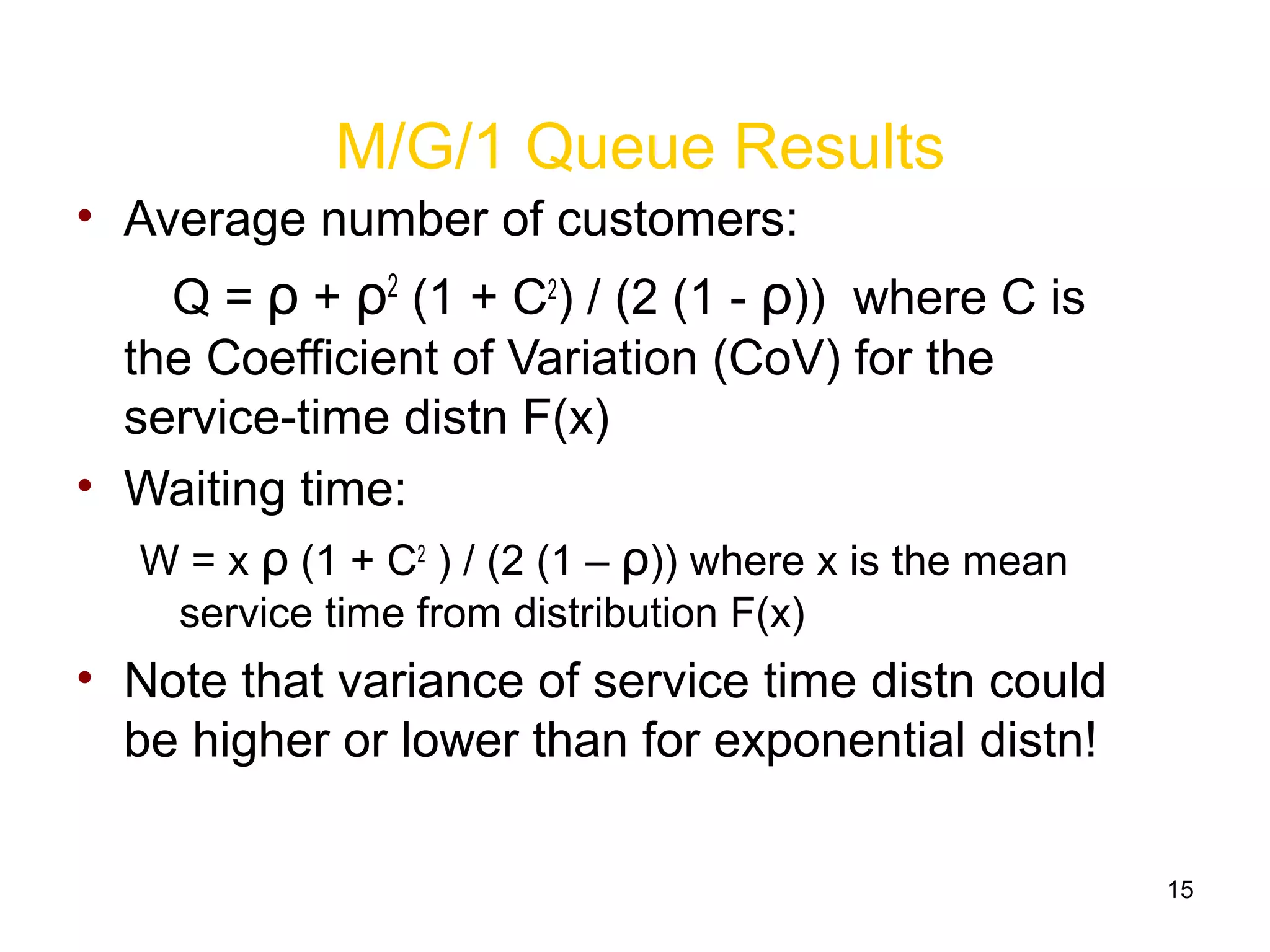
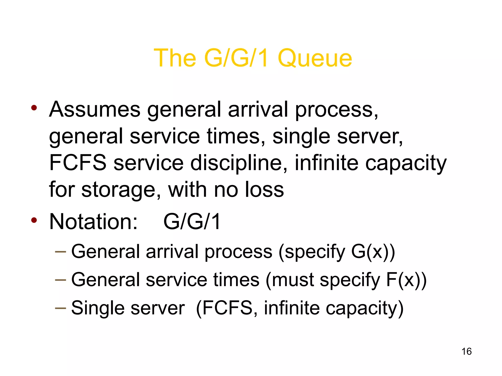
1
Queuing Theory
By
Dr.V V HaraGopal
Professor,Dept of Statistics,
Osmania University,
Hyderabad-500 007
Email Id:haragopal_vajjha@yahoo.com
2
Queueing Theory Basics
• Queueing theory provides a very general
framework for modeling systems in
which customers must line up (queue)
for service (use of resource)
– Banks (tellers)
– Restaurants (tables and seats)
– Computer systems (CPU, disk I/O)
– Networks (Web server, router, WLAN)
3
Queue-based Models
• Queueing model represents:
– Arrival of jobs (customers) into system
– Service time requirements of jobs
– Waiting of jobs for service
– Departures of jobs from the system
• Typical diagram:
Customer
Arrivals Departures
Buffer Server
4
Why Queue-based Models?
• In many cases, the use of a queuing model
provides a quantitative way to assess system
performance
– Throughput (e.g., job completions per second)
– Response time (e.g., Web page download time)
– Expected waiting time for service
– Number of buffers required to control loss
• Reveals key system insights (properties)
• Often with efficient, closed-form calculation
5
Caveats and Assumptions
• In many cases, using a queuing model has the
following implicit underlying assumptions:
– Poisson arrival process
– Exponential service time distribution
– Single server
– Infinite capacity queue
– First-Come-First-Serve (FCFS) discipline
(also known as FIFO: First-In-First-Out)
• Note: important role of memoryless property!
6
Advanced Queuing Models
• There is Lot of published work on
variations of the basic model:
– Correlated arrival processes
– General (G) service time distributions
– Multiple servers
– Finite capacity systems
– Other scheduling disciplines (non-FIFO)
• We will start with the basics!
7
Queue Notation
• Queues are concisely described using
the Kendall notation, which specifies:
– Arrival process for jobs {M, D, G, …}
– Service time distribution {M, D, G, …}
– Number of servers {1, n}
– Storage capacity (buffers) {B, infinite}
– Service discipline {FIFO, PS, SRPT, …}
• Examples: M/M/1, M/G/1, M/M/c/c
8
The M/M/1 Queue
• Assumes Poisson arrival process,
exponential service times, single server,
FCFS service discipline, infinite capacity
for storage, with no loss
• Notation: M/M/1
– Markovian arrival process (Poisson)
– Markovian service times (exponential)
– Single server (FCFS, infinite capacity)
9
The M/M/1 Queue (cont’d)
• Arrival rate: λ (e.g., customers/sec)
– Inter-arrival times are exponentially distributed
(and independent) with mean 1 / λ
• Service rate: μ (e.g., customers/sec)
– Service times are exponentially distributed
(and independent) with mean 1 / μ
• System load: ρ = λ / μ
0 ≤ ρ ≤ 1 (also known as utilization factor)
• Stability criterion: ρ < 1 (single server systems)
10
Queue Performance Metrics
• N: Avg number of customers in system
as a whole, including any in service
• Q: Avg number of customers in the
queue (only), excluding any in service
• W: Avg waiting time in queue (only)
• T: Avg time spent in system as a whole,
including wait time plus service time
• Note: Little’s Law: N = λ T
11
M/M/1 Queue Results
• Average number of customers in the
system: N = ρ / (1 – ρ)
• Variance: Var(N) = ρ / (1 - ρ)2
• Waiting time: W = ρ / (μ (1 – ρ))
• Time in system: T = 1 / (μ(1 – ρ))
12
The M/D/1 Queue
• Assumes Poisson arrival process,
deterministic (constant) service times,
single server, FCFS service discipline,
infinite capacity for storage, no loss
• Notation: M/D/1
– Markovian arrival process (Poisson)
– Deterministic service times (constant)
– Single server (FCFS, infinite capacity)
13
M/D/1 Queue Results
• Average number of customers:
Q = ρ/(1 – ρ) – ρ2
/ (2 (1 - ρ))
• Waiting time: W = x ρ / (2 (1 – ρ)) where
x is the mean service time
• Note that lower variance in service time
means less queueing occurs 
14
The M/G/1 Queue
• Assumes Poisson arrival process,
general service times, single server,
FCFS service discipline, infinite capacity
for storage, with no loss
• Notation: M/G/1
– Markovian arrival process (Poisson)
– General service times (must specify F(x))
– Single server (FCFS, infinite capacity)
15
M/G/1 Queue Results
• Average number of customers:
Q = ρ + ρ2
(1 + C2
) / (2 (1 - ρ)) where C is
the Coefficient of Variation (CoV) for the
service-time distn F(x)
• Waiting time:
W = x ρ (1 + C2
) / (2 (1 – ρ)) where x is the mean
service time from distribution F(x)
• Note that variance of service time distn could
be higher or lower than for exponential distn!
16
The G/G/1 Queue
• Assumes general arrival process,
general service times, single server,
FCFS service discipline, infinite capacity
for storage, with no loss
• Notation: G/G/1
– General arrival process (specify G(x))
– General service times (must specify F(x))
– Single server (FCFS, infinite capacity)
17
Queueing Network Models
• So far we have been talking about a
queue in isolation
• In a queueing network model, there can
be multiple queues, connected in series
or in parallel (e.g., CPU, disk, teller)
• Two versions:
– Open queueing network models
– Closed queueing network models
18
Open Queuing Network Models
• Assumes that arrivals occur externally
from outside the system
• Infinite population, with a fixed arrival
rate, regardless of how many in system
• Unbounded number of customers are
permitted within the system
• Departures leave the system (forever)
19
Closed Queuing Network Models
• Assumes that there is a finite number of
customers, in a self-contained world
• Finite population; arrival rate varies
depending on how many and where
• Fixed number of customers (N) that
recirculate in the system (forever)
• Can be analyzed using Mean Value
Analysis (MVA) and balance equations

Q theory

  • 1.
    1 Queuing Theory By Dr.V VHaraGopal Professor,Dept of Statistics, Osmania University, Hyderabad-500 007 Email Id:haragopal_vajjha@yahoo.com
  • 2.
    2 Queueing Theory Basics •Queueing theory provides a very general framework for modeling systems in which customers must line up (queue) for service (use of resource) – Banks (tellers) – Restaurants (tables and seats) – Computer systems (CPU, disk I/O) – Networks (Web server, router, WLAN)
  • 3.
    3 Queue-based Models • Queueingmodel represents: – Arrival of jobs (customers) into system – Service time requirements of jobs – Waiting of jobs for service – Departures of jobs from the system • Typical diagram: Customer Arrivals Departures Buffer Server
  • 4.
    4 Why Queue-based Models? •In many cases, the use of a queuing model provides a quantitative way to assess system performance – Throughput (e.g., job completions per second) – Response time (e.g., Web page download time) – Expected waiting time for service – Number of buffers required to control loss • Reveals key system insights (properties) • Often with efficient, closed-form calculation
  • 5.
    5 Caveats and Assumptions •In many cases, using a queuing model has the following implicit underlying assumptions: – Poisson arrival process – Exponential service time distribution – Single server – Infinite capacity queue – First-Come-First-Serve (FCFS) discipline (also known as FIFO: First-In-First-Out) • Note: important role of memoryless property!
  • 6.
    6 Advanced Queuing Models •There is Lot of published work on variations of the basic model: – Correlated arrival processes – General (G) service time distributions – Multiple servers – Finite capacity systems – Other scheduling disciplines (non-FIFO) • We will start with the basics!
  • 7.
    7 Queue Notation • Queuesare concisely described using the Kendall notation, which specifies: – Arrival process for jobs {M, D, G, …} – Service time distribution {M, D, G, …} – Number of servers {1, n} – Storage capacity (buffers) {B, infinite} – Service discipline {FIFO, PS, SRPT, …} • Examples: M/M/1, M/G/1, M/M/c/c
  • 8.
    8 The M/M/1 Queue •Assumes Poisson arrival process, exponential service times, single server, FCFS service discipline, infinite capacity for storage, with no loss • Notation: M/M/1 – Markovian arrival process (Poisson) – Markovian service times (exponential) – Single server (FCFS, infinite capacity)
  • 9.
    9 The M/M/1 Queue(cont’d) • Arrival rate: λ (e.g., customers/sec) – Inter-arrival times are exponentially distributed (and independent) with mean 1 / λ • Service rate: μ (e.g., customers/sec) – Service times are exponentially distributed (and independent) with mean 1 / μ • System load: ρ = λ / μ 0 ≤ ρ ≤ 1 (also known as utilization factor) • Stability criterion: ρ < 1 (single server systems)
  • 10.
    10 Queue Performance Metrics •N: Avg number of customers in system as a whole, including any in service • Q: Avg number of customers in the queue (only), excluding any in service • W: Avg waiting time in queue (only) • T: Avg time spent in system as a whole, including wait time plus service time • Note: Little’s Law: N = λ T
  • 11.
    11 M/M/1 Queue Results •Average number of customers in the system: N = ρ / (1 – ρ) • Variance: Var(N) = ρ / (1 - ρ)2 • Waiting time: W = ρ / (μ (1 – ρ)) • Time in system: T = 1 / (μ(1 – ρ))
  • 12.
    12 The M/D/1 Queue •Assumes Poisson arrival process, deterministic (constant) service times, single server, FCFS service discipline, infinite capacity for storage, no loss • Notation: M/D/1 – Markovian arrival process (Poisson) – Deterministic service times (constant) – Single server (FCFS, infinite capacity)
  • 13.
    13 M/D/1 Queue Results •Average number of customers: Q = ρ/(1 – ρ) – ρ2 / (2 (1 - ρ)) • Waiting time: W = x ρ / (2 (1 – ρ)) where x is the mean service time • Note that lower variance in service time means less queueing occurs 
  • 14.
    14 The M/G/1 Queue •Assumes Poisson arrival process, general service times, single server, FCFS service discipline, infinite capacity for storage, with no loss • Notation: M/G/1 – Markovian arrival process (Poisson) – General service times (must specify F(x)) – Single server (FCFS, infinite capacity)
  • 15.
    15 M/G/1 Queue Results •Average number of customers: Q = ρ + ρ2 (1 + C2 ) / (2 (1 - ρ)) where C is the Coefficient of Variation (CoV) for the service-time distn F(x) • Waiting time: W = x ρ (1 + C2 ) / (2 (1 – ρ)) where x is the mean service time from distribution F(x) • Note that variance of service time distn could be higher or lower than for exponential distn!
  • 16.
    16 The G/G/1 Queue •Assumes general arrival process, general service times, single server, FCFS service discipline, infinite capacity for storage, with no loss • Notation: G/G/1 – General arrival process (specify G(x)) – General service times (must specify F(x)) – Single server (FCFS, infinite capacity)
  • 17.
    17 Queueing Network Models •So far we have been talking about a queue in isolation • In a queueing network model, there can be multiple queues, connected in series or in parallel (e.g., CPU, disk, teller) • Two versions: – Open queueing network models – Closed queueing network models
  • 18.
    18 Open Queuing NetworkModels • Assumes that arrivals occur externally from outside the system • Infinite population, with a fixed arrival rate, regardless of how many in system • Unbounded number of customers are permitted within the system • Departures leave the system (forever)
  • 19.
    19 Closed Queuing NetworkModels • Assumes that there is a finite number of customers, in a self-contained world • Finite population; arrival rate varies depending on how many and where • Fixed number of customers (N) that recirculate in the system (forever) • Can be analyzed using Mean Value Analysis (MVA) and balance equations