Queue

1. Simple queueing models
1 M/M/1 queue
This model describes a queue with a single server which serves customers
in the order in which they arrive. Customer arrivals constitute a Poisson
process of rate λ. Recall that this means that the number of customers
arriving during a time period [t, t+s] is a Poisson random variable with mean
λs, and it is independent of the past of the arrival process. Equivalently, the
inter-arrival times (between the arrival of one customer and the next) are
iid Exponential random variables with parameter λ and mean 1/λ. Thus,
the arrival process is Markovian, which is what is denoted by the first M in
M/M/1.
The second M says that the service process is Markovian. Customer service
times are exponentially distributed, with parameter µ and mean 1/mu, and
the service times of different customers are mutually independent. By the
memoryless property of the exponential distribution, knowing how much
service a customer has already received gives us no information about how
much more service it requires. When a customer has been served, it departs
from the queue.
The 1 in M/M/1 refers to the fact that there is a single server. If there are
c servers, we call it an M/M/c queue. Customers are served in their order
of arrival. This is called the first-come-first-served (FCFS) or first-in-first-
out (FIFO) service discipline. It is not the only possible service discipline.
Other examples used in practice include processor sharing (PS) where the
server spreads its effort equally among all customers in the queue, and last-
come-first-served (LCFS). If needed, we will specify the service discipline
in force by writing M/M/1 − P S, M/M/1 − LCF S etc., taking FCFS to
be the default if nothing is specified. We assume that the queue has an
infinite waiting room, so that no arriving customers are turned away. If
1

2. there is a finite waiting room of size K, we call it an M/M/1/K queue. We
assume that the server is busy whenever there is at least one customer in the
system. Such a service discipline is called work-conserving. If the service
discipline is not work-conserving, we say that the server is on vacation, when
there is work in the system but the server isn’t working. If the customers
are jobs and the servers are machines, ‘vacactions’ could well correspond to
machine breakdowns. We won’t be studying non-work conserving queues in
this course; however, many of the techniques we learn can be extended to
them.
Let Xt denote the number of customers in the queue at time t. What
can we say about P (Xt+δ = j|Xt = i) for small δ? Suppose first that
i > 0. Then, one of two things can happen. We can either have a customer
arrival, or the customer currently in service can finish and depart. The
probability of the first event is λδ + o(δ). The probability of the second is
µδ +o(δ). With the residual probability 1−(λ+µ)δ +o(δ), the state remains
unchanged. Moreover, these probabilities are conditionally independent of
the past history of the stochastic process Xs , s ≤ t, given the current state
Xt = i. Thus, Xt , t ≥ 0 is a Markov process with the following transition
rates:
qi,i+1 = λ, qi,i−1 = µ, qi,i = −(λ + µ), ∀i ≥ 1.
Similar reasoning shows that q0,1 = λ and q0,0 = −λ. At this point, you
might want to draw an arrow diagram to represent this Markov process with
states denoting circles, and arrows between them representing transition
rates. (The arrow from a state to itself is conventionally omitted as its rate
is implicit from those of the outgoing arrows from that state.)
Observe that the Markov process Xt , t ≥ 0 is a birth-death process since
it has state space {0, 1, 2, . . .} and the only allowed transitions from state
i are to states i + 1 and i − 1. Hence, it is reversible provided it has an
invariant distribution. Let’s suppose for the moment that it has an invariant
distribution π. Then π must solve the detailed balance equations
πi qij = πj qji ∀i, j, i.e., πi λ = πi+1 µ, i = 0, 1, 2, . . . , (1)
along with the normalisation condition
∞
πi = 1. (2)
i=0
We obtain from (1) that πi = (λ/µ)πi−1 for all i ≥ 1. Hence, denoting λ/µ
2

3. by ρ, we get πi = ρi π0 . Substituting this in (2), we see that
πi = (1 − ρ)ρi , ∀i ≥ 0, if ρ < 1. (3)
If ρ ≥ 1 on the other hand, then there is no invariant distribution. Is there
an intuitive explanation of this fact?
Note that ρ ≥ 1 corresponds to λ ≥ µ. Now λ is the rate at which customers
arrive and µ is the maximum rate at which they can be served. Hence, if
ρ > 1, then work enters the system faster than it can be served, so it
tends to accumulate and the total work (total number of customers) tends
to infinity over time. In this case, we see that the queue is unstable. If
ρ < 1, then all work entering the system can be served and the queue is
stable. In this case, there is a steady state, and the invariant distribution
describes the steady state or long run behaviour of the system. If ρ = 1,
then the queue is critically loaded. If both arrival and service processes
were deterministic, then the queue would have a steady state behaviour.
However, random fluctuations cause work to gradually accumulate in the
queue, and the queue length again tends to infinity over time. Nevertheless,
the critical case is different from the unstable case in that the queue length
√
grows in proportion to t rather than t as the time t tends to infinity.
2 Performance measures
From a practical point of view, we are interested in how many customers
are typically in the queue, and how long a typical customer needs to wait
for service. Let N denote the random number of customers in the queue in
steady state, including the customer receiving service (if any). The invariant
queue length distribution computed in (3) tells us that
P (N = n) = (1 − ρ)ρn , n = 0, 1, 2, . . . . (4)
In particular, P (N = 0) = 1 − ρ. This is the probability that the queue is
empty in steady state. Equivalently, it is the fraction of time that the queue
is empty in the long run. This makes intuitive sense because work comes
into the queue at rate λ and the server can complete work at rate µ > λ.
Hence, the fraction of time that the server is busy should be λ/µ = ρ, and
the fraction of time that the server is idle (because the queue is empty)
should be 1 − ρ.
3

4. We now compute the mean number in queue from (4). The most convenient
way to do this is using generating functions. We have
∞
1−ρ
GN (z) = E[z N ] = (1 − ρ)ρn z n = ,
1 − ρz
n=0
provided |z| < 1/ρ. From this, we obtain
ρ(1 − ρ) ρ
E[N ] = GN (1) = 2
| |z=1 = . (5)
(1 − ρz) 1−ρ
Observe that the mean queue length increases to infinity as ρ increases to 1,
i.e., as the load on the queue increases to its critical value. From a practical
point of view, this effect can be quite dramatic. The mean queue length at
a load of ρ = 0.9 is 9, while at a load of ρ = 0.99, it is 99. Hence, in a nearly
criticality loaded queue, a small increase in the service rate can achieve a
huge improvement in performance!
The queue length is a measure of performance seen from the viewpoint of
the system operator. The expected waiting time (until the beginning of
service), or the expected response time or sojourn time (until the customer
departs) might be more relevant from the point of view of the customer. We
now compute this quantity.
Consider a typical customer entering the system in steady state. We will
show later that the random queue length, N , seen by a typical customer
upon arrival (in the case of Poisson arrivals) is the same as the steady state
queue length, i.e., it has the invariant queue length distribution given in (4).
Now suppose this newly arriving customer sees n customers ahead of him.
He needs to wait for all of them to complete service, and for his own service
to complete, before he can depart the system. Hence, his response time W
is given by
˜
W = S1 + S2 + S3 + . . . + Sn + Sn+1 . (6)
Here, Sn+1 is his own service time, S2 , . . . , Sn are the service times of the
˜
customers waiting in queue, and S1 is the residual service time of the cus-
tomer currently in service. Clearly, S2 , . . . , Sn+1 are iid Exp(µ) random
˜
variables, and independent of S1 . Moreover, by the memoryless property of
˜
the exponential distribution, S1 also has an Exp(µ) distribution. Hence, we
have by (6) that
µ
n+1 ( µ−θ )n+1 , if θ < µ,
E eθW N = n = E[eθS1 ] =
+∞, if θ ≥ µ.
4

5. Taking the expectation of this quantity with respect to the random variable
N , whose distribution is given by (4), we get
∞
1 − ρ µρ n+1 (1 − ρ)λ µ − θ µ−λ
E eθW = = = ,
ρ µ−θ ρ(µ − θ) µ − λ − θ µ−λ−θ
n=0
if θ < µ−λ, and E[eθW ] = ∞ if θ ≥ µ−λ. Comparing this with the moment
generating function of an exponential distribution, we see that the response
time W has an exponential distribution with parameter µ − λ. Hence, the
mean response time is
1
E[W ] = . (7)
µ−λ
Comparing this with (5), we see that
E[N ] = λE[W ]. (8)
This equality is known as Little’s law. It holds in great generality and not
just for the M/M/1 queue.
Little’s law: Let At be any arrival process, i.e., At is a counting process
counting the number of arrivals up to time t. The service times can have
arbitrary distribution, and be dependent on one another or on the arrival
times. The service discipline can be arbitrary (e.g., processor sharing or
LCFS), and there can be one or more serves. Let Nt denote the queue
length (number of customers in the system at time t) and let Wn denote
the sojourn time of the nth arriving customer. We assume only that the
following limits exist:
t n
At 1
lim = λ, lim Ns ds = N , lim Wk = W .
t→∞ t t→∞ t 0 n→∞
k=0
Then, N = λW . Note that this equality holds for every sample path of the
stochastic process for which these limits exist. If the stochastic process is
ergodic, then these limits exist (almost surely) and are equal to the corre-
sponding expectations, i.e, N = E[N ] and W = E[W ].. We haven’t defined
ergodicity but, intuitively, it is a notion of the stochastic process being well-
behaved in the sense of satisfying the law of large numbers - sample means
converge to the true mean.
A proof of this result can be found in many textbooks; see, e.g., Jean Wal-
rand, An Introduction to Queueing Networks. The intuition behind it is as
5

6. follows. Suppose each customer entering the system pays $1 per unit of time
spent in the system. So, customers pay $E[W ] on average. Since they enter
the system at rate λ, the rate at which revenue is earned is λE[W ]. On the
other hand, the system earns $n per unit time when there are n customers
in the system. Hence, the average rate at which revenue is earned is E[N ].
As these are two ways of calculating the same quantity, they must be the
same.
3 The PASTA property
In the course of computing the mean waiting time, we assumed that a typical
arrival sees the queue in its invariant distribution. At first, this may seem
an innocuous assumption, but it is by no means obvious, as the following
counterexample shows.
Consider a single-server queue into which customers arrive spaced 2 units
apart, deterministically, and suppose also that the arrival time of the first
customer is random, uniformly distributed on [0, 2]. Suppose that customers
need service for iid random times uniformly distributed between 0 and 2.
The queue length is not a continuous-time Markov process but it is never-
theless clear how it evolves. If the queue is started empty, then the queue
length becomes 1 when the first customer arrives, stays at 1 for a random
length of time of unit mean, and uniformly distributed between 0 and 2.
Thus, the queue length is guaranteed to return to zero before the next ar-
rival. This cycle repeats itself indefinitely. Now, if we consider any fixed
time, then at this time the queue is equally likely to either be empty or to
have exactly 1 customer in it. Thus, the steady state queue length distrib-
ution assigns probability 0.5 each to states 0 and 1, and probability 0 to all
other states. On the other hand, new arrivals always see an empty queue!
Thus, the queue length distribution seen by arrivals is not the same as the
steady-state queue length distribution.
However, such a situation cannot arise if the arrivals form a homogeneous
Poisson process, as in the M/M/1 queue or, indeed, in any queue with
Poisson arrivals, irrespective of the service time distribution, the service
discipline, or the number of servers. This fact is known as the PASTA
property (Poisson arrivals see time averages).
More formally, suppose that Xt , t ≥ 0 is a Markov process on some state
6

7. space S, having unique invariant distribution π. Suppose that Nt , t ≥ 0 is a
Poisson process satisfying the property that (Nu − Nt , u > t) is independent
of Xs , s ≤ t. If we think of Xt as the queue length process and Nt as
the arrival process, then this says that the arrival process is Poisson and
that future arrivals are independent of the past of the queue length process.
(Clearly, the past of the arrival process won’t be independent of the past or
current queue length.) We now have:
lim P (Xt = x|Nt+δ − Nt = 1) = P (Xt = x). (9)
δ↓0
In words, this says that knowing that there was an arrival just after time t
does not tell us anything about the queue length distribution. In particular,
if the chain is in stationarity, P (Xt = x) = πx and (9) says that the state
of the Markov process Xt just before an arrival is the same as its invariant
distribution. In other words, arrivals see the invariant distribution.
The proof of (9) is easy and follows from Bayes’ theorem. Observe that
P (Xt = x, Nt+δ − Nt = 1)
P (Xt = x|Nt+δ − Nt = 1) =
P (Nt+δ − Nt = 1)
P (Xt = x)P (Nt+δ − Nt = 1|Xt = x)
=
P (Nt+δ − Nt = 1)
P (Xt = x)P (Nt+δ − Nt = 1)
=
P (Nt+δ − Nt = 1)
= P (Xt = x).
We have used the fact that future arrivals are independent of the current
state in order to obtain the third equality above.
More generally, for any Markovian queueing system, we can compute the
queue length distribution seen at arrival or departure epochs. We now illus-
trate this with an example.
Example: M/M/1 queue with balking
This is a queue with Poisson arrivals at rate λ, exponentially distributed
job sizes with mean 1/µ and a single server, as for an M/M/1 queue. The
difference is that not all arriving customers join the queue. A customer who,
upon arrival, sees n customers ahead of him, joins the queue with probability
1 n
n+1 , and departs without service with the residual probability n+1 . Thus,
a customer who sees an empty queue is sure to join, but customers become
less and less likely to join as the queue gets longer.
7

8. The number of customers in the system evolves as a continuous time Markov
process, and it can be shown that this process is reversible (being a birth-
death chain), and has invariant distribution given by
ρn −ρ
πn = e , n = 0, 1, 2, . . .
n!
We want to compute the number of customers in queue as seen by a typical
arrival who chooses to join the queue (excluding the joining customer). We
can compute this as follows:
P (XA = n) = P (Xt = n|arrival in [t, t + dt)
P (Xt = n and arrival in [t, t + dt))
=
P (arrival in [t, t + dt))
1
πn λdt n+1
= ∞ 1
k=0 πk λdt k+1
ρn e−ρ /((n + 1)!)
= ∞ k −ρ
.
k=0 ρ e /((k + 1)!)
We have used Bayes’ theorem to get the second equality above. Now,
∞ ∞
ρk 1 ρk eρ − 1
= = .
(k + 1)! ρ k! ρ
k=0 k=1
Substituting this in the above, we get
ρn+1
P (XA = n) = .
(n + 1)!(eρ − 1)
Note that this is different from πn , demonstrating once again that, if the
arrival process isn’t Poisson, then a typical arrival need not see the system
in its stationary distribution.
We can similarly compute the distribution seen by departures in stationarity.
The probability that a departing customer leaves behind n customers in
8

9. queue is given by
P (XD = n) = P (Xt = n + 1|departure in [t, t + dt)
P (Xt = n + 1 and departure in [t, t + dt))
=
P (departure in [t, t + dt))
πn+1 µdt
= ∞
k=1 πk µdt
ρ n+1 e−ρ /((n + 1)!)
=
1 − π0
ρn+1
= .
(n + 1)!(eρ − 1)
Note that this is the same as P (XA = n). This is true of any queue where
arrivals and departures happen singly rather than in batches because you
can match up arriving and departing customers in such a way that, for every
customer who enters a queue with n customers, there is a departure that
leaves behind n customers in the queue.
4 Departure process from an M/M/1 queue
If an M/M/1 queue has arrival rate λ which is strictly smaller than the ser-
vice rate µ, then the queue is stable and doesn’t build up an infinite backlog.
Consequently, all arrrivals eventually depart, and the mean departure rate
is the same as the arrival rate, λ. But what can we say about the depar-
ture process? The answer is given by the following theorem, which is called
Burke’s theorem.
Theorem 1 The departure process from an M/M/1 queue with arrival rate
λ strictly smaller than the service rate µ, is also a Poisson process of rate
λ in equilibrium. Moreover, the past of the departure process is independent
of the current state.
Proof. The proof is a pretty straightforward application of reversibility.
Note that the queue length process Xt is reversible in equilibrium since it is a
birth-death Markov process. Arrivals correspond to upward jumps of Xt and
departures to downward jumps. Now, the time reveral of Xt has the same
probabilistic properties as Xt itself, but arrivals in forward time correspond
9

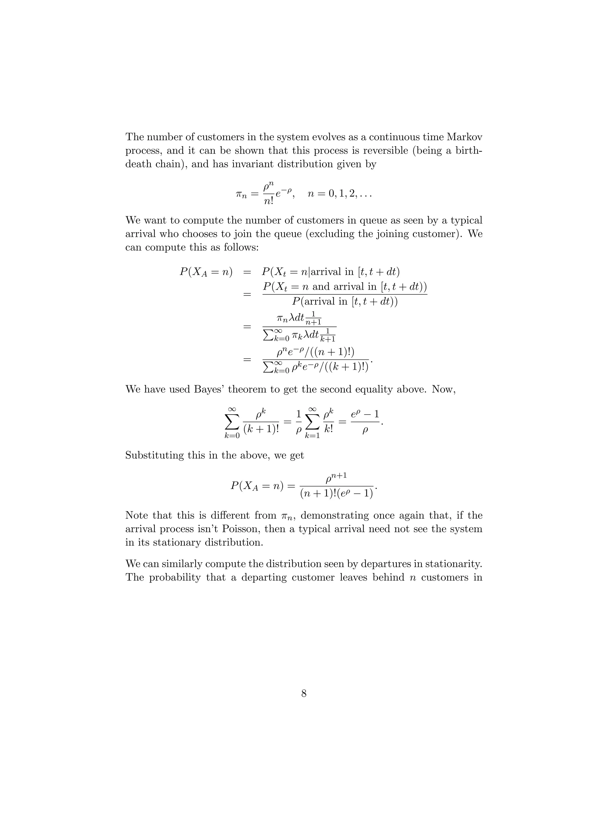
10. to departures in reversed time and vice versa. Hence, the departure process
for the forward time process should have the same probability law as the
arrival process for its time reversal. But this is a Poisson process because
the time reversal is indistinguishable from the original process.
Likewise, the past of the departure process in forward time corresponds to
the future of the arrival process in reversed time, which we know to be
independent of the current state since this arrival process is Poisson.
5 M/M/c and M/M/∞ queues
Recall that the first M says that the arrival process is Poisson, the second
M that the service times are exponential, and the number refers to the
number of servers, which is either a given number c or infinite. While
real queues rarely have infinitely many servers, this can often be a good
approximation when the number of servers is large! It was first introduced
to model telephone exchanges, where the number of available lines may run
into the tens of thousands. In systems with a large number of servers, it
can often be a matter of judgement whether to model it as an M/M/c or
M/M/∞ queue.
Customers are held in a common queue and sent to the first server that be-
comes available. If one or more are already free when they enter the system,
they go to one of these servers at random. As the service time distribution
is the same at every server, it doesn’t matter how ties are broken.
Let Xt denote the number of customers in the system at time t. If Xt ≤ c,
then Xt servers are busy serving these customers (in parallel), and the re-
maining c−Xt servers are idle. If Xt > c, then all servers are busy, and Xt −c
customers are waiting in queue. The possible transitions of this system are
that a new customer could arrive, or an existing customer could complete
service and leave. The probability of two or more customers leaving simulta-
neously is zero, as we shall see. The probability that a new customer arrives
in the interval [t, t + δ] is λδ + o(δ), independent of the past, since the arrival
process is Poisson with rate λ. The probability that an existing customer
departs in the interval [t, t + δ] is the probability that one of the min{Xt , c}
customers currently being served completes its service in that interval. This
probability is µδ + o(δ) for each of these customers, independent of the past
(because service requirements are exponentially distributed, with parameter
10

11. µ), and of one another (since service requirements of different customers are
mutually independent). Hence, the probability that exactly one of them
departs is
1 − (1 − µδ + o(δ))min{Xt ,c} = min{Xt , c}µδ + o(δ),
while the probability that two or more depart is o(δ). Thus, the departure
probability in [t, t + δ] depends only on the current state Xt , and on no
further details of the past. In other words, Xt , t ≥ 0 is a continuous time
Markov process, with transition rates:
µi, 0 ≤ i ≤ c,
qi,i+1 = λ, qi,i−1 = qi,i = −λ − µ min{i, c}.
µc, i > c
Note that all the statements in the paragraph above also hold if c is replaced
by ∞.
Let us now compute the invariant distributions of these queues, starting
with the M/M/∞ queue. As the number in system is a birth-death Markov
process, it is reversible if it has an invariant distribution, and the invariant
distribution π satisfies the detailed balanced equations, which are as follows:
λπi = µ(i + 1)πi+1 , i ≥ 0.
ρ
Let ρ = λ/µ. Then, we can rewrite the above as πi+1 = i+1 πi , which implies
ρi
that πi = i! π0 .
This can be normalised to be a probability distribution, for
any ρ, if we choose π0 = e−ρ . Hence, the invariant distribution of the
M/M/∞ queue is given by
ρi
πi = e−ρ , (10)
i!
which we recognise as the Poisson distribution with parameter ρ. Note
that this queue is stable for any combination of arrival rates and (non-zero)
service rates. As there are infinitely many servers, the total service rate
exceeds the total arrival rate once the number in system becomes sufficiently
large.
The mean of a Poisson(ρ) random variable is ρ. (Verify this for yourself.)
Hence, the mean number in an M/M/∞ queue is given by E[N ] = ρ. We
can also see this intuitively, as follows. The number of busy servers at any
time is the same as the number of customers in the system as there are
always enough servers available. Hence, the mean rate at which servers are
11

12. doing work is the mean number of busy servers, which is also the mean
number of customers in the system. On the other hand, the mean rate at
which work is brought into the system is the mean arrival rate, λ, times
the mean amount of work brought by each customer, 1/µ, which is ρ. This
should be the same, in equilibrium, as the mean rate at which work is done.
Therefore, the mean number of customers in the system should be ρ.
Next, by Little’s law, the mean sojourn time of a customer is E[W ] =
E[N ]/λ = 1/µ. This is again intuitive. On average, a customer brings in
1/µ amount of work, and doesn’t need to wait as there is always a server
available. Hence, his sojourn time is the same as his own service requirement.
Next, we compute the invariant distribution of the M/M/c queue. Again,
the queue length process is a birth-death Markov process, and so, if the de-
tailed balance equations have a solution which is a probability distribution,
then that is the invariant distribution of the Markov process. The detailed
balance equations are
λπi = µ min{i + 1, c}πi+1 , i ≥ 0,
which have the solution
ρi
πi = i! π0 , i < c,
(11)
ρc ρ i−c
c! c π0 , i ≥ c,
∞
where ρ = λ/µ. We want to choose π0 so as to make i=0 πi = 1, i.e.,
c−1 ∞ c−1 ∞
1 ρi ρc ρ i−c ρi ρc ρ j
= + = + . (12)
π0 i! c! c i! c! c
i=0 i=c i=0 j=0
There is a non-zero solution for π0 if and only if the above sum is finite,
which happens if and only if ρ < c. If ρ ≥ c, the detailed balance equations
have no solution which is a probability distribution. This result is intuitive
because the maximum rate at which work can be done in the M/M/c queue
is c, and if the rate ρ at which work enters the system is greater than this,
then the queue is unstable and the waiting times build up to infinity. If
ρ < c, then the invariant distribution is given by (11) with π0 being given
by the solution of (12). The solution can’t be simplified further. The mean
queue size and mean waiting time can easily be computed numerically from
the invariant distribution, but there are no closed form expressions for them.
12

13. 6 M/G/1 queues: Pollaczek-Khinchin formula
So far, we have only considered queues with Poisson arrivals and exponen-
tially distributed service requirements. That is because it is only in those
cases that the queue length process is Markovian, which makes the analysis
of such systems tractable. If either the inter-arrival times, or the service
times, or both, weren’t exponential, then the future evolution of the queue
length would depend not only on the current queue length, but on how much
time has elapsed since the last arrival or service completion, as this affects
the residual time to the next arrival/ service completion. (In the exponen-
tial case, there is no such dependence because of the memoryless property
of the exponential distribution.) As a result, the analysis of such systems
is far from straightforward, and we will not deal with them in this course,
with a few exceptions.
The first exception is the M/G/1 queue or, more precisely, the M/G/1 −
F IF O queue, where we make it explicit that the service discipline is first-
in-first-out or first-come-first-served. The G here stands for general, which
means that we allow arbitrary service time distributions. We will still as-
sume, though, that the service requirements of different customers are iid.
As this system is more complicated, we will not aim to derive its invari-
ant distribution, but content ourselves with finding the mean queue length
and mean waiting time. The formulas for these quantities are called the
Pollaczek-Khinchin (henceforth abbreviated as P-K) formulas.
In the following, we consider an M/G/1 queue where arrivals occur according
to a Poisson process of rate λ, service times are iid with general distribution,
there is a single server operating a FIFO policy, and there is infinite waiting
room. We denote the mean service time by 1/µ and define ρ = λ/µ to be
consistent with the notation used so far for the M/M/1 queue. We shall
assume that ρ < 1, so that the queue is stable and does not blow up to
infinity. We now aim to find an expression for the mean sojourn time in this
queue.
Define the following quantities:
Si : service time required by customer i
Ri : residual service requirement of customer in service when i arrives
Ni : number of customers in system when customer i arrives
Wi : sojourn time of customer i in system
13

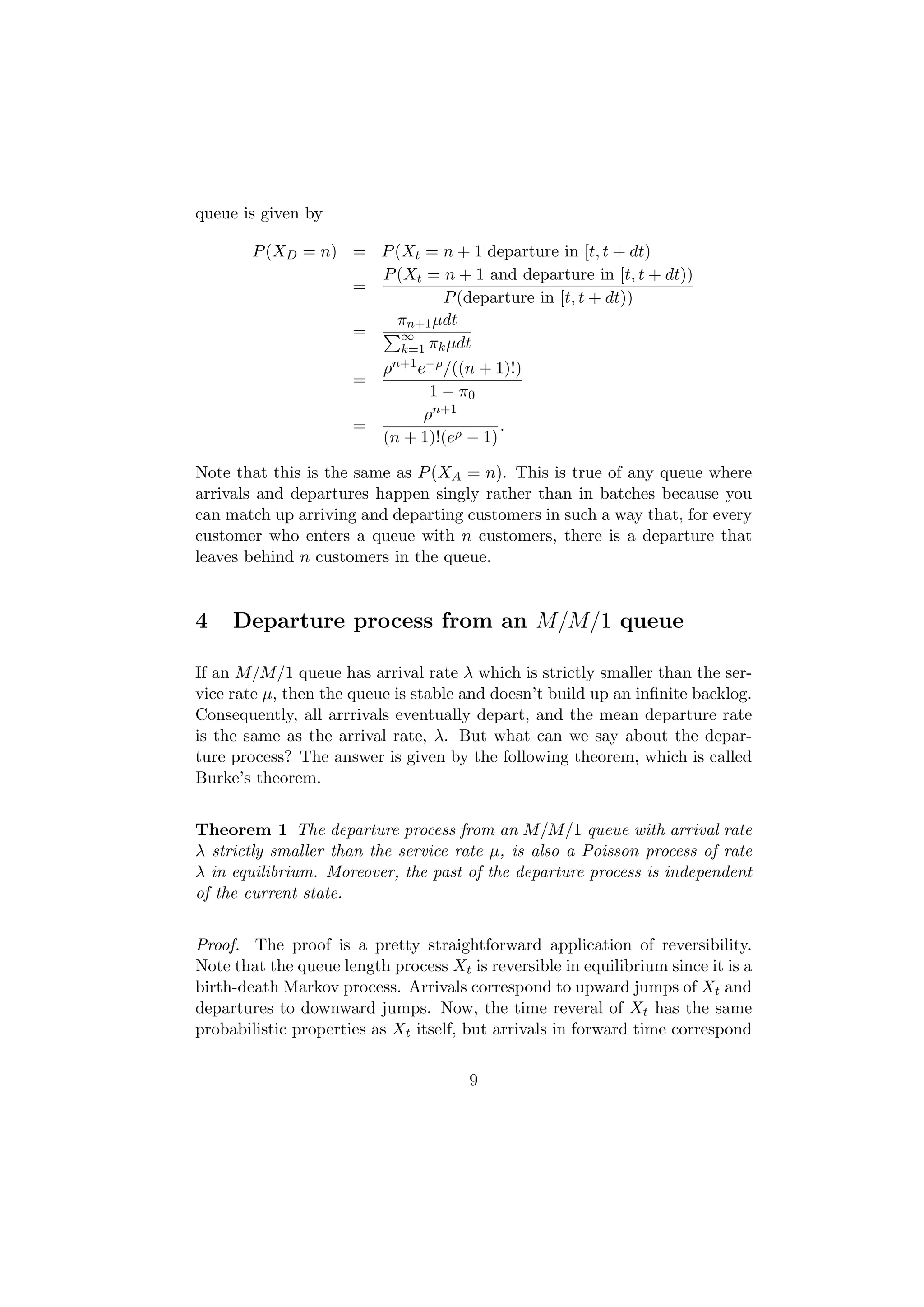
14. We take Ri to be zero if customer i enters an empty queue. We have
Ni −1
W i = Si + R i + Si−j 1(Ni ≥ 1).
j=1
If Ni = 1, then the sum above is empty, and we take it to be zero. Taking
expectations in the above equation, we have
Ni −1
E[Wi ] = E[Si ] + E E Ri 1(Ni ≥ 1) Ni E E Si−j Ni
j=1
= E[Si ] + P (Ni ≥ 1)E[Ri |Ni ≥ 1] + E[S1 ]E[(Ni − 1)1(Ni ≥ 1)].
We have used the linearity of expectation and the independence of the fu-
ture service times Si−j from Ni to obtain the second equality above. Now,
E[Ni 1(Ni ≥ 1)] = E[Ni ], so we can rewrite the above as
E[W ] = E[S] + P (N ≥ 1)E[R|N ≥ 1] + E[S](E[N ] − P (N ≥ 1)). (13)
We have dropped subscripts for notational convenience, keeping in mind
that we are referring to quantitites in steady state, and hence that these
don’t depend on the index i.
Now, N is a random variable denoting the number of customers in system
seen by the typical arrival. The arrival process into the M/G/1 queue is a
Poisson process by assumption and so, by the PASTA property, N has the
same distribution as the number of customers in system in stationarity (or
in steady state or equilibrium - we use these terms interchangeably). Hence,
applying Little’s law, we have E[N ] = λE[W ]. Substituting this in (13),
and noting that λE[S] = λ/µ = ρ, we get
(1 − ρ)E[W ] = P (N ≥ 1)E[R|N ≥ 1] + E[S](1 − P (N ≥ 1)). (14)
It remains to compute P (N ≥ 1) and E[R|N ≥ 1].
First, we note that customers enter the queue at rate λ, each bringing a
random amount of work with them, with mean 1/µ. Thus, the average rate
at which work comes into the system is λ/µ = ρ. This must be the same as
the average rate at which work is completed because the system is stable,
meaning that no huge backlog of work builds up. Now, the server works at
unit rate whenever the queue is non-empty, which means that the long-run
fraction of time that the queue is non-empty has to be ρ. In other words,
14

15. P (N ≥ 1) = ρ. (If that argument is not persuasive enough, you can prove
this along the same lines as the proof of Little’s law. Assume that each
customer is charged $1 per unit time whenever it is at the head of the queue
and is being served. Thus, a customer with job size S ends up paying $ S.
But customers enter the system at rate λ, so the rate at which money is
paid into the system is λE[S] = ρ dollars per unit time. On the other hand,
the server earns $ 1 per unit time whenever it is working, i.e., whenever the
queue is non-empty. As the rate at which the server earns money has to
match the rate at which customers are paying it in, the fraction of time the
server is busy has to be ρ.) Thus, we can rewrite (14) as
(1 − ρ)E[W ] = ρE[R|N ≥ 1] + (1 − ρ)E[S]. (15)
Next, we compute E[R|N ≥ 1], the mean residual service time of the cus-
tomer at the head of the queue at the arrival instant of a typical customer,
conditional on the queue not being empty at this time. Let us look at a
very long interval of the time axis, so the time interval [0, T ] for some very
large T . The fraction of this interval occupied by the service of customers
whose total service requirement is in (x, x + dx) is λxfS (x)dx where fS (x) is
the density of the service time distribution evaluated at x. (We are making
somewhat loose statements involving the infinitesimals dx, but these can be
made precise.) To see this, note that approximately λT customers arrive
during this time, of which a fraction fS (x)dx have service requirement in
(x, x + dx), and each of them occupies an interval of the time axis of size
x when it gets to the head of the queue. The fraction of the interval [0, T ]
occupied by the service of some customer (i.e., the fraction that the system
∞
is non-empty) is then given by 0 λxfS (x)dx = λE[S].
Now, the typical arrival conditioned to enter a non-empty system is equally
likely to arrive any time during a busy period. (Though this might seem
obvious, it is actually a subtle point and relies on the arrival process being
Poisson.) Hence, the probability density for the typical arrival to enter the
system during the service of a customer whose total job size is x is given
by xfS (x)/E[S]. Moreover, the arrival occurs uniformly during the service
period of this customer and hence sees a residual service time of x , on 2
average. Thus, the mean residual service time seen by a typical arrival who
enters a non-empty system is
∞
1 x E[S 2 ]
E[R|N ≥ 1] = xfS (x)dx = . (16)
E[S] 0 2 2E[S]
15

16. Substituting this in (15), we get
ρ E[S 2 ] λE[S 2 ]
E[W ] = E[S] + = E[S] + . (17)
1 − ρ 2E[S] 2(1 − ρ)
We have used the fact that ρ = λ/µ = λE[S] to obtain the last equality.
The formula for the mean sojourn time above consists of two terms, the first
of which is the customer’s own service time, and the second is the mean
waiting time until reaching the head of the queue. Applying Little’s law to
the above formula, we also get
λ2 E[S 2 ]
E[N ] = λE[W ] = ρ + . (18)
2(1 − ρ)
The formulas (17,18) are referred to as the Pollaczek-Khinchin (PK) for-
mulas for the mean of the queue size and sojourn time. There are also PK
formulas for the moment generating functions of these quantities, but we will
not be studying them in this course. The goal of this section was to intro-
duce you to some of the methods that can be used to study non-Markovian
queues. We will see another such example in the next section. However,
but for these two exceptions, we will be restricting ourselves to Markovian
queueing models in this course.
7 M/G/∞ queue
This is a model of a queueing system with Poisson arrivals, general iid service
times, and infinitely many servers. Thus, an arriving job stays in the system
for a period equal to its own service time and then departs. We denote the
arrival rate by λ and the mean service time by 1/µ. The system is stable
for all λ and µ.
Note that the number of customers in the system is not a Markov process
since the past of this process contains information about when customers
arrived, and hence potentially about how much longer they will remain in
the queue. This is easiest to see if all the job sizes are deterministically
equal to 1/µ. Thus, the methods we learnt for analysing Markov processes
are not relevant. Instead, we shall use techniques from the theory of point
processes.
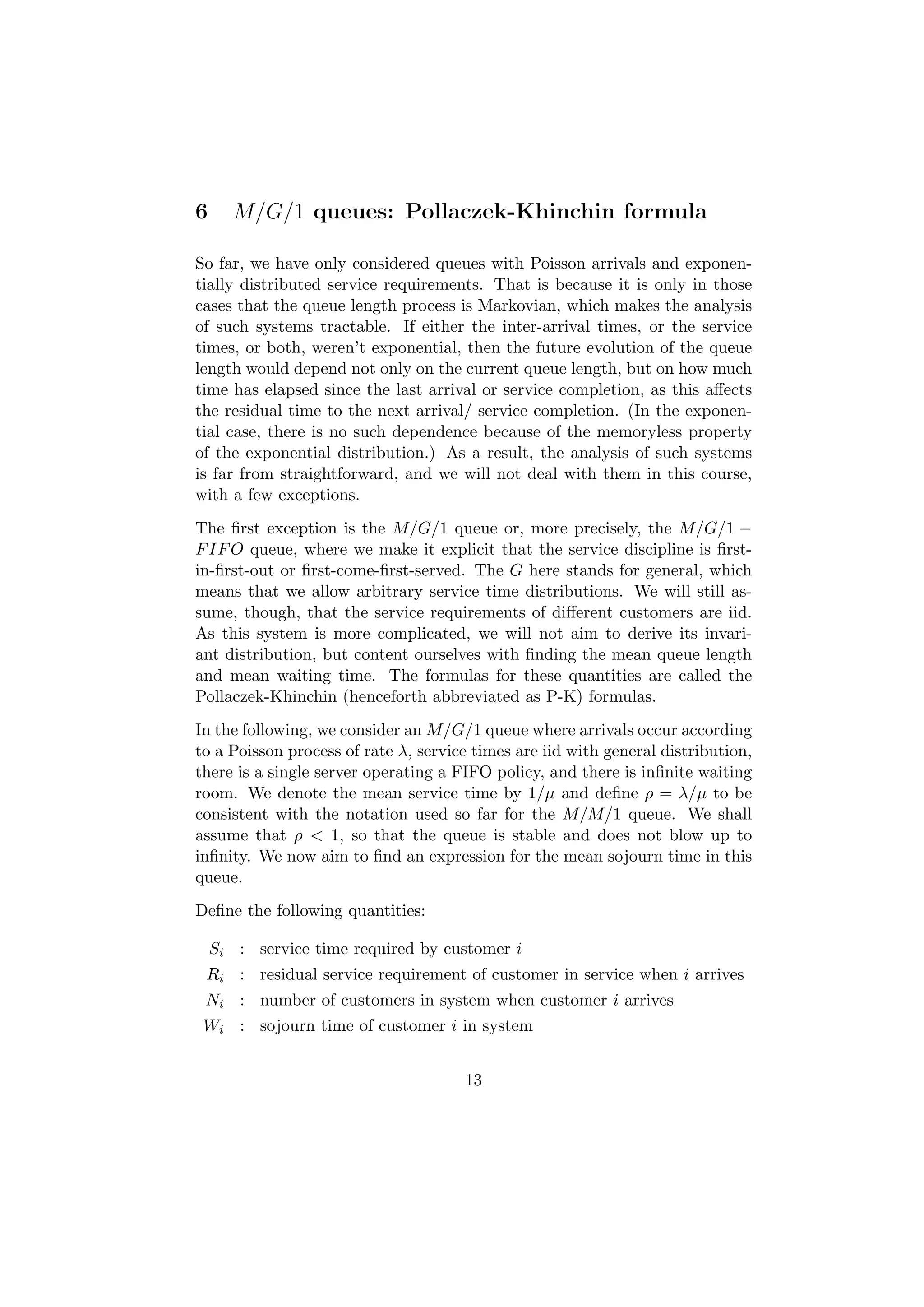
Definition A stochastic process on Rn is called a point process if, with
each (measurable) set A ⊆ Rn , it associates a non-negative discrete random
16

17. variable NA , and that the collection of random variables {NA , A ⊆ R} satisfy
the following properties:
1. N∅ = 0.
∞
2. If A1 , A2 , A3 , . . . are disjoint, and A = ∪∞ Aj , then NA =
j=1 j=1 NAj .
Observe that we already saw an example of a point process on R, namely
the Poisson process. If N· satisfies properties 1 and 2 above, it is called a
measure. If, in addition, it takes values in the whole numbers, it is called
a counting measure. Thus, a point process can be thought of as a random
counting measure. More concretely, you can think of it as a collection of
randomly placed points, with NA denoting the random number of points in
a set A. Note that the points need not be placed independently.
Definition A point process on Rn is said to be a Poisson process with
intensity function λ(·) if the following statements hold:
1. If A and B are disjoint subsets of Rn , then NA and NB are independent
random variables.
2. For any set A, NA has the Poisson distribution with mean A λ(x)dx.
Here dx = dx1 dx2 · · · dxn denotes the infinitesimal volume element in
Rn .
The Poisson process is said to be homogeneous if the intensity function is a
constant, i.e., λ(x) = λ for all x ∈ Rn . Note that, as for Poisson processes
on the real line, the second property above can be rephrased as saying that
the probability of having a point in a small neighbourhood around x is
approximately λ(x) times the volume of the neighbourhood, and that this
is independent of the location of all other points.
Now, consider such a Poisson point process on R×[0, ∞) with intensity func-
tion λ(x, y) = λfS (y), where λ denotes the arrival rate into the M/G/∞
queue and fS denotes the density of the service time distribution. We inter-
pret a point at (x, y) as denoting the arrival of a customer at time x with
job size y. Note that the intensity has been chosen to correctly model the
arrival rate and job size distribution.
Consider a realisation of this Poisson point process. Say we want to know
X0 , the number of jobs in the system at time 0. A job that entered the
17

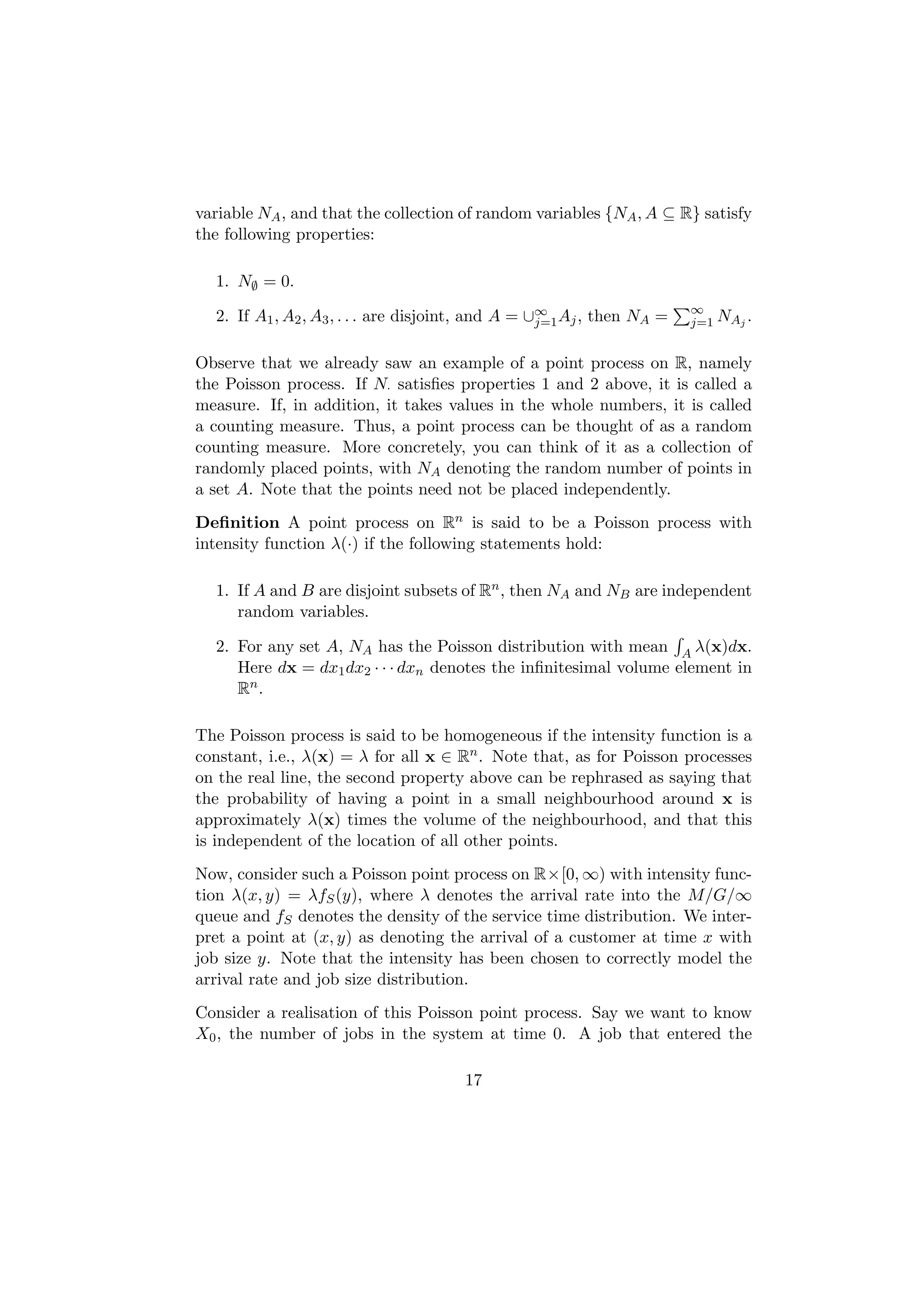
18. system at time −t will still be in the system at time zero if and only if its
job size is smaller than t. Thus, the set of all jobs that are in the system at
time zero can be identified with the set of points that lie in the triangular
region A = {(x, y) : x ≤ 0, y > −x}. But, by the property of a Poisson
process, the number of such points is a Poisson random variable with mean
∞ 0
η = λ(x, y)dxdy = λfS (y)dxdy
A y=0 x=−y
∞
= λ yfS (y)dy = λE[S].
y=0
We have thus shown that the number of jobs in the system at time zero
has a Poisson distribution with mean ρ = λ/µ. We defined the system on
the time interval (inf ty, ∞), so that by time zero, or by any finite time,
the system has reached equilibrium. Hence, the invariant distribution of the
number of jobs in the system is Poisson(ρ).
Recall that this is the same as the invariant distribution for an M/M/∞
queue with the same arrival rate and mean service time. Thus, the invari-
ant distribution depends on the service time distribution only through its
mean. We call this the insensitivity property as the invariant distribution is
insensitive to the service time distribution.
Besides the M/G/∞ queue, the M/G/1 − LIF O and M/G/1 − P S queues
(with servers employing the last-in-first-out and processor sharing service
disciplines respectively) also exhibit the insensitivity property. In their case,
the invariant distribution is geometric, just like the M/M/1 queue with the
same arrival rate and mean service time. We will not prove this fact, but
will make use of it, so it is important to remember it.
18